Epsilon Expansion and One-Loop Scaling

The previous page found the upper critical dimension of the Ising universality class. In the continuum scalar theory

$$S[\phi] = \int d^D x\, \left[ {1\over2}(\partial\phi)^2 +{1\over2}r\phi^2 +{\lambda\over4!}\phi^4 +\cdots \right],$$

the quartic coupling has engineering dimension

$$[\lambda]=4-D.$$

For $D>4$, the quartic perturbation is irrelevant at the Gaussian fixed point, and mean-field theory is asymptotically correct. For $D<4$, it is relevant, so the Gaussian fixed point cannot describe the true long-distance critical theory. The borderline case $D=4$ is special: the coupling is classically marginal, and loop integrals generate logarithms.

The epsilon expansion turns this borderline into a controlled calculation. Write

$$D=4-\epsilon, \qquad 0<\epsilon\ll1.$$

Then the quartic coupling is weakly relevant. Classical scaling makes it grow at long distances, but one-loop fluctuations reduce it. The two effects balance at an interacting infrared fixed point, the Wilson–Fisher fixed point. Since the fixed-point coupling is proportional to $\epsilon$, perturbation theory becomes an expansion around an interacting, non-Gaussian theory.

Required background. Critical propagators and the upper critical dimension supplies the continuum propagator, self-energy power counting, and the identification $D_c=4$ for $\phi^4$ theory.

Helpful background. Hubbard–Stratonovich fields and the continuum limit explains how the Ising order parameter becomes a scalar field and why its mass is a temperature-like coupling.

Logarithms at four dimensions

Infrared RG time and quartic-coupling normalization

Throughout this page $D$ is the Euclidean dimension of the statistical system. We use the one-component Ising normalization

$$S[\phi]=\int d^D x\, \left[ {1\over2}(\partial\phi)^2 +{1\over2}r\phi^2 +{\lambda\over4!}\phi^4 -h\phi \right].$$

The $\mathbb Z_2$ spin-flip symmetry is $\phi\mapsto-\phi$ when $h=0$. The parameter $r$ is the temperature-like coupling. In a cutoff theory, criticality is not the bare equation $r=0$; rather, $r$ must be tuned to a critical surface $r=r_c(\lambda)$. Below, $r$ denotes the shifted scaling variable unless the distinction matters.

We use the infrared RG time

$$\ell=\log b,$$

where $b>1$ is a length rescaling factor. Thus increasing $\ell$ means flowing toward longer distances. In the dimensionless coupling

$$g={3\lambda\over16\pi^2}\,\mu^{-\epsilon},$$

with momentum scale $\mu$, the one-loop momentum-scale beta function is

$$\mu {dg\over d\mu}=-\epsilon g+g^2+O(g^3).$$

Equivalently, in the long-distance convention used most often on this page,

$${dg\over d\ell}=\epsilon g-g^2+O(g^3).$$

The numerical coefficient in the definition of $g$ is a normalization choice. Fixed-point coordinates depend on that choice and on the renormalization scheme; critical exponents computed consistently do not.

The one-loop correction to the quartic vertex contains the massless bubble integral, evaluated at nonzero Euclidean external momentum $p$,

$$B_D(p)=\int_q {1\over q^2(q+p)^2}, \qquad \int_q\equiv\int {d^Dq\over(2\pi)^D},$$

where $p$ is a characteristic external momentum. By power counting,

$$B_D(p)\sim p^{D-4}.$$

Equivalently, with a UV cutoff $\Lambda$, the ultraviolet part behaves as

$$B_D(p)\sim \int^{\Lambda}dq\,{q^{D-1}\over q^4} =\int^{\Lambda}dq\,q^{D-5}.$$

Thus $D=4$ is logarithmic:

$$B_4(p)\sim K_4\log{\Lambda\over p}+\text{finite}, \qquad K_4={1\over8\pi^2}$$

for a spherical momentum shell. The finite part depends on the scheme and on the external momentum configuration. The logarithm does not. It is the signal that a coupling measured at one scale differs from the coupling measured at another scale.

For the interaction $\lambda\phi^4/4!$, the local one-loop correction to the four-point vertex is

$$\delta\lambda_{\rm loop} =-{3\over2}\lambda^2 \int_{\rm shell}{d^Dq\over(2\pi)^D}{1\over(q^2+r)^2}+\text{higher-derivative terms}.$$

The factor $3$ counts the $s$, $t$, and $u$ channels. The factor $1/2$ is the bubble symmetry factor in this normalization. At criticality and in four dimensions,

$$\delta\lambda_{\rm loop} =-{3\lambda^2\over16\pi^2}d\ell.$$

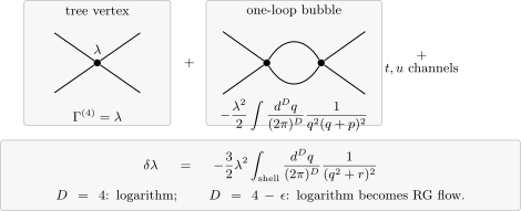
The one-loop correction to the four-point vertex is the bubble diagram in the three channels. Its logarithm at $D=4$ becomes the beta function near $D=4-\epsilon$.

The same logarithm appears in dimensional regularization as a pole. Introduce a reference scale $\mu$ and define

$$B_D(p;\mu) =\mu^{4-D}\int {d^Dq\over(2\pi)^D}{1\over q^2(q+p)^2},$$

so that the regulated integral is dimensionless, as it is at $D=4$. A standard Feynman-parameter evaluation gives

$$B_D(p;\mu) = \mu^{4-D} {1\over(4\pi)^{D/2}} {\Gamma(2-D/2)\Gamma(D/2-1)^2\over\Gamma(D-2)} (p^2)^{D/2-2}.$$

Near $D=4-\epsilon$,

$$B_{4-\epsilon}(p;\mu) = {1\over16\pi^2} \left[ {2\over\epsilon}-\log {p^2\over\mu^2} +\text{scheme-dependent constant}+O(\epsilon) \right].$$

The pole and the logarithm are two representations of the same marginal short-distance sensitivity.

Momentum shells and the Wilsonian step

The Wilsonian RG makes the logarithm into a differential equation. Split the field into slow and fast Fourier modes,

$$\phi(x)=\phi_<(x)+\phi_>(x),$$

where

$$|q|<\Lambda/b \quad\text{for }\phi_<, \qquad \Lambda/b<|q|<\Lambda \quad\text{for }\phi_>,$$

with $b=e^{d\ell}$. Define the slow-field effective action by

$$e^{-S_{\rm eff}[\phi_<]} = \int D\phi_>\,e^{-S[\phi_<+\phi_>]}.$$

After integrating over the thin shell, rescale momenta, coordinates, and fields to restore the cutoff:

$$q'=bq, \qquad x'=x/b, \qquad \phi'(x')=b^{(D-2)/2}\phi_<(x).$$

The field rescaling keeps the Gaussian kinetic term normalized.

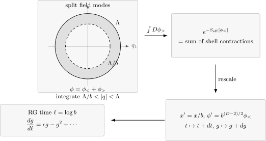
A Wilsonian step integrates out fast modes in the shell $\Lambda/b<|q|<\Lambda$, then rescales lengths and fields to restore the cutoff. Repeating this operation turns couplings into functions of the observation scale.

For the shell calculation, introduce the cutoff-scaled coupling

$$\bar\lambda=\lambda\Lambda^{-\epsilon}.$$

Its classical flow follows from $[\lambda]=\epsilon$:

$$\bar\lambda\mapsto b^\epsilon\bar\lambda, \qquad \left.{d\bar\lambda\over d\ell}\right|_{\rm tree} =\epsilon\bar\lambda.$$

The loop correction at criticality uses

$$\int_{\rm shell}{d^Dq\over(2\pi)^D}{1\over q^4} =K_D\int_{\Lambda/b}^{\Lambda}dq\,q^{D-5},$$

where

$$K_D={S_{D-1}\over(2\pi)^D}, \qquad S_{D-1}={2\pi^{D/2}\over\Gamma(D/2)}.$$

In $D=4-\epsilon$, the shell integral is

$$K_D\Lambda^{-\epsilon}d\ell+O(d\ell^2).$$

Therefore, near four dimensions,

$${d\bar\lambda\over d\ell} = \epsilon\bar\lambda -{3\bar\lambda^2\over16\pi^2} +O(\bar\lambda^3,\epsilon\bar\lambda^2),$$

where $K_D$ has been expanded about $K_4=1/(8\pi^2)$. In terms of

$$g={3\bar\lambda\over16\pi^2},$$

the one-loop infrared beta function is

$$\boxed{ {dg\over d\ell}=\epsilon g-g^2+O(g^3). }$$

This is the simplest form of the Wilson–Fisher beta function for the one-component Ising scalar.

The Wilson–Fisher fixed point

The fixed points of

$$\beta_R(g)={dg\over d\ell}=\epsilon g-g^2$$

are

$$g=0, \qquad g_*=\epsilon.$$

The Gaussian point is unstable below four dimensions, because

$$\beta_R'(0)=\epsilon>0.$$

A small positive quartic coupling grows as the system is viewed at longer distances. The interacting fixed point is stable in the quartic direction, because

$$\beta_R'(g_*)= \epsilon-2g_*=-\epsilon.$$

Thus, if $g(\ell)=g_*+\delta g(\ell)$, then

$${d\delta g\over d\ell}=-\epsilon\delta g+O(\delta g^2,\epsilon^2\delta g),$$

so

$$\delta g(\ell)\sim e^{-\epsilon\ell}.$$

The corresponding correction-to-scaling exponent is

$$\omega=\epsilon+O(\epsilon^2).$$

In terms of the cutoff-scaled quartic coupling,

$$\bar\lambda_* ={16\pi^2\over3}\epsilon+O(\epsilon^2).$$

The corresponding dimensionful coupling is $\lambda_*=\bar\lambda_*\Lambda^\epsilon$ in this cutoff convention; it is not itself a universal fixed-point coordinate. The dimensionless value is small when $\epsilon$ is small, which is what makes the expansion controlled.

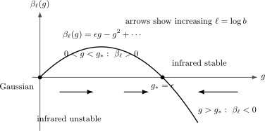
For the length-scale flow $dg/d\ell=\epsilon g-g^2$, the Gaussian fixed point becomes unstable for $D<4$, while the Wilson–Fisher fixed point $g_*=\epsilon$ is stable in the quartic-coupling direction.

The one-loop flow equation is exactly solvable:

$${dg\over d\ell}=g(\epsilon-g).$$

For initial value $g(0)=g_0>0$,

$$\boxed{ g(\ell)= {\epsilon\over1+\left({\epsilon\over g_0}-1\right)e^{-\epsilon\ell}}. }$$

For $0<g_0<\epsilon$, the coupling grows toward $\epsilon$. For $g_0>\epsilon$, it decreases toward $\epsilon$. Thus the fixed point attracts a range of microscopic quartic couplings. This is the field-theoretic expression of universality.

At $\epsilon=0$, the same equation becomes

$${dg\over d\ell}=-g^2,$$

so

$$g(\ell)={g_0\over1+g_0\ell}.$$

Since $\ell\sim\log(R/a)$, the four-dimensional coupling vanishes only as $1/\log R$. This is why four-dimensional mean-field behavior is modified by logarithms rather than by new leading power laws.

The mass direction and the exponent ν

The Wilson–Fisher fixed point is not stable in every direction. The mass or temperature perturbation must still be tuned. Write the temperature-like scaling field as $t$, proportional to $T-T_c$ after a nonuniversal normalization. Under RG,

$${dt\over d\ell}=y_t t+\text{nonlinear terms}.$$

At the Gaussian fixed point, $y_t=2$. Interactions renormalize the composite operator $\phi^2$. The tadpole shell displays both the additive and multiplicative effects:

$${\lambda\over2} \int_{\rm shell}{d^Dq\over(2\pi)^D}{1\over q^2+r} = {\lambda\over2} \int_{\rm shell}{d^Dq\over(2\pi)^D} \left({1\over q^2}-{r\over q^4}+\cdots\right).$$

The first term moves the critical surface to $r_c(\lambda)$. After subtracting that additive shift, the term linear in the scaling field $t=r-r_c$ combines with the tree-level rescaling. In the normalization above, the one-loop flow is

$${dt\over d\ell} = \left(2-{g\over3}+O(g^2)\right)t.$$

Evaluating this at the Wilson–Fisher fixed point gives

$$\boxed{ y_t=2-{\epsilon\over3}+O(\epsilon^2). }$$

The correlation length exponent is the inverse of this relevant eigenvalue:

$$\nu={1\over y_t}.$$

Therefore

$$\boxed{ \nu={1\over2}+{\epsilon\over12}+O(\epsilon^2). }$$

This is the first non-mean-field exponent produced by the epsilon expansion. The Gaussian answer $\nu=1/2$ is shifted because the energy operator, represented in the continuum by $\phi^2$, has an anomalous scaling dimension at the interacting fixed point.

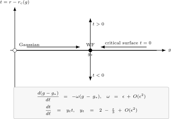
The Wilson–Fisher fixed point is stable along the quartic-coupling direction but unstable along the temperature direction. Criticality is reached by tuning onto the critical surface $r=r_c(g)$.

Why η starts at two loops

The anomalous dimension $\eta$ is defined by the critical two-point function

$$\langle\phi(x)\phi(0)\rangle \sim {1\over |x|^{D-2+\eta}},$$

or, equivalently,

$$G(k)\sim {1\over k^{2-\eta}}.$$

At one loop in $\phi^4$ theory, the self-energy is the tadpole

$$\Sigma_1(k)={\lambda\over2}\int_q {1\over q^2+r}.$$

This integral is independent of the external momentum $k$. It shifts the mass and therefore the location of the critical surface, but it does not renormalize the coefficient of $k^2$ in the inverse propagator. Hence

$$\boxed{ \eta=0+O(\epsilon^2). }$$

The first momentum-dependent self-energy correction is the two-loop sunset diagram:

$$\Sigma_2(k) \sim \lambda^2 \int {d^Dp\,d^Dq\over p^2q^2(p+q+k)^2}.$$

Dimensional analysis at criticality gives

$$\Sigma_2(k)-\Sigma_2(0) \sim \lambda^2 k^{2D-6}.$$

At $D=4$, this becomes $\lambda^2 k^2\log(\Lambda/k)$ after subtracting local terms. Since $g_*\sim\epsilon$, the resulting field anomalous dimension begins at order $\epsilon^2$.

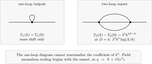
The tadpole is independent of external momentum and shifts only the critical mass. The two-loop sunset is the first momentum-dependent self-energy correction, so the anomalous dimension $\eta$ begins at order $\epsilon^2$.

For the one-component Ising theory,

$$\eta={\epsilon^2\over54}+O(\epsilon^3),$$

but this two-loop number is beyond the one-loop logic of this page.

Scaling forms and first exponents

At a fixed point, the scaling dimension of the spin field is

$$\Delta_\phi={D-2+\eta\over2}.$$

The two-point function at criticality is therefore

$$\langle\phi(x)\phi(0)\rangle \sim {1\over |x|^{2\Delta_\phi}} ={1\over |x|^{D-2+\eta}}.$$

Away from criticality, the correlation length is set by the relevant temperature perturbation:

$$\xi\sim |t|^{-1/y_t}=|t|^{-\nu}.$$

The susceptibility is the integral of the connected two-point function up to distances of order $\xi$:

$$\chi \sim \int^{\xi}d^Dx\,{1\over |x|^{D-2+\eta}} \sim \xi^{2-\eta}.$$

Thus

$$\gamma=\nu(2-\eta).$$

Using $\eta=0+O(\epsilon^2)$ and $\nu=1/2+\epsilon/12+O(\epsilon^2)$ gives

$$\boxed{ \gamma=1+{\epsilon\over6}+O(\epsilon^2). }$$

Other exponents follow from scaling relations. To first order,

$$\begin{aligned} \eta&=0+O(\epsilon^2),\\ \nu&={1\over2}+{\epsilon\over12}+O(\epsilon^2),\\ \gamma&=1+{\epsilon\over6}+O(\epsilon^2),\\ \beta_{\rm mag}&={1\over2}-{\epsilon\over6}+O(\epsilon^2),\\ \delta&=3+\epsilon+O(\epsilon^2),\\ \alpha&={\epsilon\over6}+O(\epsilon^2). \end{aligned}$$

Here $\beta_{\rm mag}$ is the magnetization exponent, not inverse temperature and not an RG beta function. The notation is old and unfortunate, so context has to do the work.

Setting $\epsilon=1$ gives rough three-dimensional Ising estimates such as

$$\nu\approx0.583, \qquad \gamma\approx1.167.$$

These are not precision values. The achievement of the one-loop epsilon expansion is structural: it explains why a non-Gaussian universal fixed point exists and why its exponents can be computed systematically.

A gauge-coupling analogy

The same dimensional reasoning appears in gauge theory. In the convention $F=dA+[A,A]$, where the coupling multiplies the whole action, a $D$-dimensional Euclidean Yang–Mills action is

$$S_{\rm YM}={1\over4g_D^2}\int d^D x\,F_{\mu\nu}^aF_{\mu\nu}^a.$$

The gauge coupling has engineering dimension

$$[g_D^2]=4-D.$$

Thus four dimensions are also the dimension where Yang–Mills coupling is classically marginal. At $D=4$, loops generate logarithmic running. In $D=3$, the coupling $g_3^2$ has dimension of mass, so the natural dimensionless coupling at momentum scale $q$ is

$$g_{\rm eff}^2(q)\sim {g_3^2\over q}.$$

It grows in the infrared already by dimensional analysis. This does not make scalar criticality and gauge dynamics identical, but it highlights a shared lesson: the physical strength of an interaction is the dimensionless coupling at the scale being probed, not the bare constant by itself.

Summary

At $D=4$, the Ising quartic coupling is classically marginal and the one-loop four-point diagram produces logarithms. Slightly below four dimensions, these logarithms combine with classical scaling to produce the beta function

$${dg\over d\ell}=\epsilon g-g^2+O(g^3), \qquad \epsilon=4-D.$$

There are two nearby fixed points:

$$g=0, \qquad g_*=\epsilon+O(\epsilon^2).$$

The Gaussian point is unstable for $D<4$. The Wilson–Fisher point is stable in the quartic direction and controls the ordinary Ising critical point. The mass direction remains relevant, with eigenvalue

$$y_t=2-{\epsilon\over3}+O(\epsilon^2).$$

Therefore

$$\nu={1\over2}+{\epsilon\over12}+O(\epsilon^2).$$

The one-loop self-energy is momentum independent, so

$$\eta=0+O(\epsilon^2).$$

The susceptibility exponent follows from scaling:

$$\gamma=1+{\epsilon\over6}+O(\epsilon^2).$$

The epsilon expansion is not a perturbation of the lattice coupling. It is an expansion in the fixed-point value of a dimensionless long-distance coupling, which is small when $D$ is close to four.

Common pitfalls

Confusing the critical mass with the bare mass. The critical condition is not the naive bare equation $r=0$. Tadpoles shift the critical surface, so one must tune the physical inverse correlation length to zero.

Forgetting the RG-time convention. With increasing momentum scale $\mu$, the beta function is $\mu\,dg/d\mu=-\epsilon g+g^2+\cdots$. With increasing length scale $\ell$, its sign is reversed. The fixed points agree, but the flow arrows do not.

Treating $\eta=0$ at one loop as exact. The one-loop tadpole is momentum independent. Wavefunction renormalization starts with the two-loop sunset, giving $\eta=O(\epsilon^2)$.

Using $\epsilon=1$ as precision perturbation theory. The expansion is controlled near four dimensions. First-order three-dimensional estimates are structural guides, not precision values.

Equating irrelevant with disposable. Above four dimensions the quartic coupling is dangerously irrelevant: it does not change the leading Gaussian critical two-point function, but it stabilizes the ordered phase and causes violations of naive hyperscaling.

Exercises

Exercise 1: Bubble power counting

Show that the bubble integral

$$B_D(p)=\int {d^Dq\over(2\pi)^D}{1\over q^2(q+p)^2}$$

has scaling dimension $D-4$.

Solution

Rescale $q=pQ$, where $p$ denotes the magnitude of the external momentum. Then

$$d^Dq=p^D d^DQ, \qquad q^2=p^2Q^2, \qquad (q+p)^2=p^2(Q+\hat p)^2.$$

Therefore

$$B_D(p) =p^{D-4} \int {d^DQ\over(2\pi)^D}{1\over Q^2(Q+\hat p)^2}.$$

The remaining integral is dimensionless after regularization. Hence

$$B_D(p)\sim p^{D-4}.$$

At $D=4$, the power vanishes and the dimensionless integral becomes logarithmic.

Exercise 2: Fixed points and their stability

For the one-loop length-scale beta function

$${dg\over d\ell}=\epsilon g-g^2,$$

find the fixed points and determine their stability for $\epsilon>0$.

Solution

Set the beta function to zero:

$$0=g(\epsilon-g).$$

Thus

$$g=0, \qquad g_*=\epsilon.$$

The derivative is

$$\beta_R'(g)=\epsilon-2g.$$

At $g=0$,

$$\beta_R'(0)=\epsilon>0,$$

so a small positive coupling grows as $\ell$ increases. The Gaussian fixed point is infrared-unstable. At $g_*=\epsilon$,

$$\beta_R'(g_*)=-\epsilon<0,$$

so deviations decay as $e^{-\epsilon\ell}$. The Wilson–Fisher fixed point is infrared-stable in the quartic direction.

Exercise 3: Integrating the one-loop flow

Solve

$${dg\over d\ell}=g(\epsilon-g)$$

with $g(0)=g_0>0$.

Solution

Separate variables:

$${dg\over g(\epsilon-g)}=d\ell.$$

Since

$${1\over g(\epsilon-g)}={1\over\epsilon}\left({1\over g}+{1\over\epsilon-g}\right),$$

integration gives

$${1\over\epsilon}\log{g\over\epsilon-g}=\ell+C.$$

Using $g(0)=g_0$ and solving for $g(\ell)$,

$$\boxed{ g(\ell)= {\epsilon\over1+\left({\epsilon\over g_0}-1\right)e^{-\epsilon\ell}}. }$$

Thus $g(\ell)$ approaches $\epsilon$ for every positive initial coupling in this one-loop approximation.

Exercise 4: The correlation-length exponent

Using

$$y_t=2-{\epsilon\over3}+O(\epsilon^2),$$

derive

$$\nu={1\over2}+{\epsilon\over12}+O(\epsilon^2).$$

Solution

By definition,

$$\nu={1\over y_t}.$$

Write

$$y_t=2\left(1-{\epsilon\over6}+O(\epsilon^2)\right).$$

Then

$$\nu={1\over2}\left(1-{\epsilon\over6}+O(\epsilon^2)\right)^{-1}.$$

Using $(1-x)^{-1}=1+x+O(x^2)$ gives

$$\nu={1\over2}\left(1+{\epsilon\over6}+O(\epsilon^2)\right) ={1\over2}+{\epsilon\over12}+O(\epsilon^2).$$

Exercise 5: Momentum dependence of the sunset

Estimate the momentum dependence of the two-loop sunset self-energy at criticality:

$$\Sigma_2(k) \sim \lambda^2\int {d^Dp\,d^Dq\over p^2q^2(p+q+k)^2}.$$

Solution

The two loop measures contribute dimension $2D$. The three propagators contribute dimension $-6$. After subtracting the $k=0$ part, the only external scale is $k$. Therefore

$$\Sigma_2(k)-\Sigma_2(0) \sim \lambda^2 k^{2D-6},$$

up to logarithms at special dimensions. At $D=4$, this is proportional to $\lambda^2k^2$ times a logarithm. This is why wavefunction renormalization, and hence $\eta$, begins at order $\lambda^2$ or $\epsilon^2$.

References

• K. G. Wilson and M. E. Fisher, “Critical Exponents in 3.99 Dimensions,” Physical Review Letters 28 (1972), 240–243, doi:10.1103/PhysRevLett.28.240.
• K. G. Wilson and J. Kogut, “The Renormalization Group and the $\epsilon$ Expansion,” Physics Reports 12 (1974), 75–199, doi:10.1016/0370-1573(74)90023-4.

Further reading

• D. J. Amit and V. Martín-Mayor, Field Theory, the Renormalization Group, and Critical Phenomena: Graphs to Computers, 3rd ed., World Scientific, Singapore, 2005.
• J. Cardy, Scaling and Renormalization in Statistical Physics, Cambridge Lecture Notes in Physics, vol. 5, Cambridge University Press, Cambridge, 1996.
• J. Zinn-Justin, Quantum Field Theory and Critical Phenomena, 4th ed., International Series of Monographs on Physics, vol. 113, Oxford University Press, Oxford, 2002.