

One-Loop Divergences and Power Counting
The previous pages built the scattering formalism: exact propagator poles define particles, LSZ reduction amputates the external legs, and QED tree diagrams give concrete amplitudes constrained by gauge invariance. The next obstacle is ultraviolet behavior. A loop diagram asks us to sum over virtual momenta of arbitrarily short wavelength. The question is not merely whether an integral is large; the real question is whether its short-distance part has the form of a local term already present in the action.
This page introduces the practical logic of perturbative renormalization at one loop. QED is the main example because it displays the important features in a protected setting: electron self-energy, photon vacuum polarization, and vertex corrections are divergent by naive momentum counting, but gauge invariance sharply restricts what those divergences can be. The result is the key bridge to renormalization: amplitudes written in terms of bare parameters depend on the cutoff, while amplitudes written in terms of physical mass, charge, and field normalizations can be cutoff independent order by order.
The final part of the page abstracts the lesson into power counting. In four spacetime dimensions, local operators of dimension below, equal to, or above four behave very differently. This is the beginning of the distinction between renormalizable interactions and effective interactions.
Three kinds of terms should be separated. A power divergence, such as , is highly regulator dependent. A logarithmic divergence controls scale dependence and survives as a pole in dimensional regularization. A nonanalytic term, such as or a threshold square root, is not a local counterterm; it describes propagation at finite momentum. For timelike momenta, the logarithm also carries the boundary prescription inherited from the Feynman integral.
Bare parameters and physical amplitudes
Section titled “Bare parameters and physical amplitudes”Start from QED in the schematic bare form
with a gauge-fixing term left implicit. The subscript reminds us that these are bare quantities: they are the parameters and fields appearing in the cutoff theory. They are not yet the physical electron mass or measured electric charge.
A scattering amplitude computed with a cutoff has the schematic form
At one loop this expression usually contains terms such as , and with some regulators also powers of . The physical claim of renormalizability is that the cutoff dependence can be absorbed into a finite set of parameter and field redefinitions:
where is a reference scale used to define the renormalized parameters. At fixed bare theory, an exact physical prediction is independent of this arbitrary scale: the running parameters and the explicit dependence of the loop corrections cancel. A prediction truncated at a finite perturbative order generally retains dependence of the first omitted order. Dependence on physical external momenta is a different matter and remains observable; see the Callan–Symanzik derivation.
Here regulator removal refers to the ultraviolet regulator. Renormalizing QED does not by itself remove infrared singularities from exclusive on-shell amplitudes. The UV discussion can be made with infrared regulation or suitable off-shell kinematics; measurable charged-particle rates also require the soft-photon inclusiveness described in infrared-finite QED.
A convenient way to display this is to write
and to define the vertex renormalization by
Equivalently,
These definitions ensure that, after the field redefinitions, the coefficients left over beyond the canonically normalized renormalized Lagrangian are exactly , , , and . Writing only would miss the factor of multiplying the bare mass term.
The constants and are chosen order by order so that specified physical normalization conditions hold. In QED, the Ward–Takahashi identity implies the important relation
when the regulator and subtraction scheme preserve gauge invariance. Together with the preceding definition, this gives in four-dimensional cutoff notation. This equality is the perturbative version of the statement that charge renormalization is tied to photon-field renormalization rather than being an arbitrary independent correction to the vertex. In the common notation , the Ward identity fixes ; dimensional regularization also supplies the conventional power of the subtraction scale needed away from four dimensions.
The one-loop QED subgraphs
Section titled “The one-loop QED subgraphs”The first divergent structures in QED are the electron self-energy, the photon self-energy, and the vertex correction. A four-photon fermion box is also superficially logarithmically divergent by naive power counting. Its possible local divergence is independent of external momenta. In the complete four-photon amplitude, the sum over inequivalent external-photon orderings must satisfy a Ward identity on every photon leg; a momentum-independent term cannot do so. The ultraviolet divergences therefore cancel in that sum. An individual box ordering need not be ultraviolet finite or transverse. Power counting identifies a possible divergence; symmetry constrains the complete amplitude.
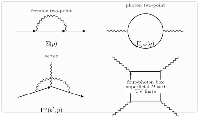
The basic one-loop QED subgraphs, shown schematically. The symbol denotes the superficial degree of divergence. Naive power counting flags all four topologies as potentially divergent. Gauge invariance restricts the actual local divergences to the QED counterterms already present in the Lagrangian. The four-photon panel represents one ordering; ultraviolet finiteness holds after summing the inequivalent external-photon orderings.
The electron self-energy has the schematic Feynman-gauge form. With the electron vertex convention of the previous page the vertex is ; the overall sign depends on the precise definition of , but the allowed divergent structures do not:
For large , the loop has one fermion propagator and one photon propagator. Naively,
looks linearly divergent. In dimensional regularization, or in the -symmetric Euclidean integral specified above, the odd term does not generate a local divergence, and the remaining divergent part has the form
with regulator-dependent constants . The two allowed structures are exactly the local operators
Thus the electron self-energy renormalizes the fermion field and the mass.
The same convention warning applies to the vertex correction: its exact overall sign is less important here than the fact that its local divergent part must be proportional to the original current operator. The vertex correction has the form
where the one-loop part is schematically
At large , the integral behaves as
so the divergence is logarithmic. Its local part is proportional to the same operator that appears in the original QED interaction:
Gauge invariance relates this divergence to the wavefunction divergence in the electron self-energy. That is the diagrammatic content of .
A useful bookkeeping table is
The table should be read as an operator statement, not as a list of regulator-independent numerical coefficients. The canonical one-loop QED calculation gives the explicit coefficient and Ward-identity checks in a declared regularization scheme.
Vacuum polarization and transversality
Section titled “Vacuum polarization and transversality”The photon self-energy, or vacuum polarization, is the fermion loop with two external photons:
A naive large- estimate gives
which suggests a quadratic divergence. But a quadratic divergence in the photon two-point function would be a local mass term
That term is not gauge invariant. In gauge-invariant renormalization, the Ward identity enforces
Therefore the divergent part must be transverse:
This is precisely the momentum-space form of the local operator
Thus vacuum polarization renormalizes the photon kinetic term and hence the electric charge. It does not give the photon a mass.
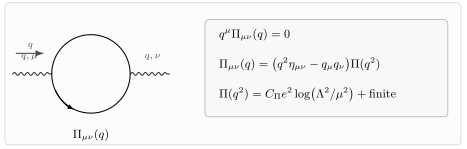
The vacuum polarization tensor is transverse: . Its logarithmic divergence has the form , so it renormalizes rather than producing a photon mass.
A good way to remember the distinction is this: the cutoff integral may look quadratically divergent before symmetry is imposed, but the divergent local operator must be legal. Gauge invariance is a veto power over counterterms.
Locality of ultraviolet divergences
Section titled “Locality of ultraviolet divergences”Why are the divergent pieces local? At large loop momentum , external momenta are small perturbations. A typical integrand can be expanded in powers of :
The divergent part comes from finitely many terms in this large- expansion. Each term is a polynomial in the external momenta multiplied by a divergent integral. A polynomial in momenta is the Fourier transform of a local differential operator. For example,
corresponds in position space to a combination of local terms such as
This is the basic reason counterterms work. The divergent part of a loop diagram does not remember the long-distance details of the process. It looks like a point interaction.
There is a caveat. A diagram that is superficially convergent can contain a divergent subdiagram. For example, a large graph may contain a self-energy insertion hidden inside it. Power counting the whole graph is not enough. The full renormalization theorem requires subtracting divergent subgraphs as well as the overall divergence. In this course, we use the one-loop examples to understand the mechanism before the all-orders formalism.
Superficial degree of divergence
Section titled “Superficial degree of divergence”For a connected QED diagram, let
- be the number of loops,
- the number of internal fermion lines,
- the number of internal photon lines,
- the number of external fermion lines,
- the number of external photon lines,
- the number of QED vertices.
At large loop momentum,
The superficial degree of divergence is therefore
The QED vertex has two fermion half-lines and one photon half-line, so
For a connected graph,
Eliminating , we obtain the QED power-counting formula
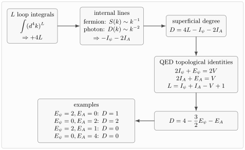
Power counting assigns for each loop integral, for each internal fermion propagator, and for each internal photon propagator. For QED this gives , before Ward identities and subdiagram structure are imposed.
This formula gives the following first warnings:
The table is deliberately called a warning rather than a verdict. The photon self-energy is not actually allowed to contain a photon mass divergence; the four-photon amplitude is not allowed to contain a local counterterm. Symmetry improves the actual ultraviolet behavior.
This distinction is not pedantry. Superficial power counting tells us which local structures could appear before imposing identities. Renormalization asks the sharper question: which local structures are compatible with all symmetries and field redefinitions? The legal answer in QED is the finite list of gauge-invariant counterterms, not every tensor one can write using .
For scalar theory in four dimensions, the analogous formula is simpler. With no derivatives at the vertex and scalar propagators behaving as , one finds
where is the number of external scalar legs. Thus the vacuum energy, two-point function, and four-point function are superficially divergent, while amplitudes with six or more external scalar legs are superficially convergent. That is why theory needs counterterms for the vacuum energy, mass, field normalization, and quartic coupling, but not an independent counterterm in four dimensions.
Engineering dimensions and operator classification
Section titled “Engineering dimensions and operator classification”Power counting can be stated without drawing any particular diagram. In four spacetime dimensions, the action is dimensionless and
The free scalar kinetic term gives
The free Dirac kinetic term gives
The Maxwell term gives
so
If a local operator has engineering dimension , then the coefficient in
has dimension
This leads to the Gaussian fixed-point classification:
The diagram compares the dimensions of operators before their coefficients are included. For example, and have dimensions two and three; their mass coefficients bring the corresponding Lagrangian terms to dimension four. The dimension-six operator instead needs a coefficient of dimension minus two.
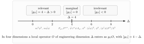
In four spacetime dimensions, an operator of engineering dimension has coefficient dimension . Near the Gaussian fixed point, dimensionless relevant couplings grow toward the infrared; marginal couplings can acquire logarithmic running, and irrelevant interactions are suppressed at low energy by powers of a heavy scale. The classification is schematic and uses operator dimensions, not the dimension of the full coefficient-times-operator term.
Examples in four dimensions include
Thus
has dimensionless and is marginal by engineering dimension. The QED coupling is also dimensionless because
By contrast, the Fermi four-fermion operator has dimension six:
Its coefficient must scale as for some heavy mass scale . Loops in such a theory generate more and more higher-dimensional counterterms. This does not make the theory useless; it means it is an effective theory with a finite range of validity.
Counterterms as a finite list
Section titled “Counterterms as a finite list”The one-loop QED divergences are local and gauge constrained. Therefore they can be absorbed into
In a linear covariant gauge, Abelian Faddeev–Popov ghosts decouple. Gauge fixing still determines the photon propagator and the gauge-dependent coefficients of the electron self-energy and vertex correction; it is not absent from these calculations. The displayed expression gives the matter and photon counterterms, with the gauge-fixing sector handled separately. The important point is the finite list and the Ward relation tying its coefficients together.
A non-gauge-invariant cutoff may appear to generate terms like
Such a term is not an independent physical parameter of unbroken QED. With a gauge-breaking regulator, a local symmetry-restoring counterterm may be needed to cancel it. The final renormalized photon two-point function must satisfy the Ward identity and contain no explicit photon mass. Dimensional regularization with the vector current treated consistently preserves transversality directly. The canonical symmetry-restoration discussion distinguishes a removable regulator artifact from a genuine anomaly.
In scalar theory, by contrast, a mass divergence
is legal unless a symmetry forbids it. This is why scalar masses are sensitive to short-distance physics in a way protected gauge-boson masses are not. That observation will become central in later discussions of naturalness and effective field theory, even though the present course only introduces the first renormalization ideas.
Example: superficial divergence in φ⁴ theory
Section titled “Example: superficial divergence in φ⁴ theory”Consider a connected diagram in four dimensions. Let be the number of internal lines, the number of quartic vertices, the number of loops, and the number of external scalar lines. Since each loop integral contributes powers of momentum and each internal scalar propagator contributes ,
The topological identities are
Therefore
Using ,
This derivation is short, but it contains the whole power-counting idea. The two-point function has , so it can have mass and kinetic divergences. The four-point function has , so it can have logarithmic coupling divergences. The six-point function has , so it is superficially convergent. If a divergent six-point subdiagram appears inside a larger graph, it must come from lower-point subdivergences already handled by lower-dimensional counterterms.
Summary
Section titled “Summary”Ultraviolet divergences in perturbative QFT are not random infinities. At high loop momentum, external momenta and masses can be expanded in powers of and . The divergent terms are polynomials in external momenta, hence local in position space. Renormalization works because these local terms can be absorbed into local counterterms.
In QED, one-loop divergences appear in the electron self-energy, vacuum polarization, and vertex correction. Gauge invariance constrains their form. The photon self-energy must be transverse, so it renormalizes rather than generating a photon mass. The vertex and electron wavefunction divergences are related by the Ward identity. After expressing amplitudes in terms of physical parameters, cutoff dependence is removed order by order.
Power counting organizes this structure. In four dimensions, operators with are relevant, are marginal, and are irrelevant near the free-field fixed point. Renormalizable theories require only a finite set of counterterms because their interactions have nonnegative infrared importance and do not force an infinite tower of new independent UV-sensitive parameters at each order. Effective field theory keeps the irrelevant operators too, but organizes them as a controlled expansion in powers of energy over a heavy scale.
Common pitfalls
Section titled “Common pitfalls”Do not confuse superficial divergence with actual divergence. Ward identities, antisymmetry, symmetric integration, and the absence of a legal local counterterm can reduce or eliminate the actual UV divergence.
Do not trust a hard cutoff blindly in a gauge theory. A regulator that violates gauge invariance can produce gauge-forbidden artifacts, such as a fake photon mass term. The final counterterms must respect the symmetries of the theory.
Do not say that a nonrenormalizable operator is meaningless. It is nonrenormalizable in the old strict sense, but in modern language it is an irrelevant operator in an effective field theory and is perfectly useful below its cutoff scale.
Do not forget subdivergences. A graph with negative overall superficial degree of divergence can still contain a divergent subgraph.
Do not interpret the absence of a power divergence in dimensional regularization as the absence of short-distance sensitivity. Dimensional regularization hides power divergences, but symmetry and operator analysis still decide which relevant parameters must be tuned or measured.
Exercises
Section titled “Exercises”Exercise 1 — Dimensions of fields and QED operators
Section titled “Exercise 1 — Dimensions of fields and QED operators”In four dimensions, use the kinetic terms to find , , and . Then determine the dimensions of the operators , , , and .
Solution
The Lagrangian density has dimension and .
For the scalar kinetic term,
so
For the Dirac kinetic term,
Since ,
For the Maxwell term,
so . Since ,
Then
and
Thus , the QED vertex, and are dimension-four Lagrangian terms, while is a dimension-six operator whose coefficient has dimension .
Exercise 2 — QED superficial degree of divergence
Section titled “Exercise 2 — QED superficial degree of divergence”Derive
for connected QED diagrams. Assume that every vertex has two fermion half-lines and one photon half-line.
Solution
The loop momentum estimate is
because each loop integral contributes , each internal fermion propagator contributes , and each internal photon propagator contributes .
The line-counting identities are
The connected graph relation is
Substitute this into :
Using
we get
The terms cancel:
Exercise 3 — Why the photon mass counterterm is forbidden
Section titled “Exercise 3 — Why the photon mass counterterm is forbidden”Suppose the vacuum polarization contained a divergent local term proportional to . Show that this would correspond to a photon mass term and explain why the Ward identity forbids it.
Solution
A local term in the photon two-point function proportional to corresponds in position space to
with . This is a photon mass term.
The Ward identity requires
If
then
which is not zero for general . Therefore the Ward identity forbids such a term. The allowed divergent structure is instead transverse:
which renormalizes the Maxwell kinetic term .
Exercise 4 — Renormalizable versus effective interactions
Section titled “Exercise 4 — Renormalizable versus effective interactions”Classify the following four-dimensional operators as relevant, marginal, or irrelevant by engineering dimension:
Solution
Using
we find
Thus is relevant, is marginal by engineering dimension, and is irrelevant.
For the QED current coupling,
so it is marginal by engineering dimension.
Finally,
so the four-fermion interaction is irrelevant in four dimensions. Its coefficient has dimension , as in Fermi theory.
Further reading
Section titled “Further reading”- Coleman, Sidney. Lectures of Sidney Coleman on Quantum Field Theory. Edited by Bryan Gin-ge Chen, David Derbes, David Griffiths, Brian Hill, Richard Sohn, and Yuan-Sen Ting. World Scientific, 2019. DOI.
- Srednicki, Mark. Quantum Field Theory. Cambridge University Press, 2007. DOI.
- Weinberg, Steven. The Quantum Theory of Fields, Volume I: Foundations. Cambridge University Press, 1995. DOI.
- Zee, A. Quantum Field Theory in a Nutshell. 2nd ed. Princeton University Press, 2010. Publisher.