

Time Ordering, Contact Terms, and Green Functions
The Dyson expansion is written with the time-ordering symbol because interaction-picture operators at different times do not generally commute. This page explains a deceptively small point that becomes one of the main engines of perturbative QFT: when derivatives act on time-ordered products, they also act on the step functions hidden inside . The resulting delta functions are called contact terms.
Those delta-functions are not optional bookkeeping. They are the reason a time-ordered two-point function is a Green function rather than a homogeneous solution of the free equation of motion. The free operator satisfies . Nevertheless, applying that differential operator outside differentiates the ordering step functions at . Their contact term produces the source in the Green-function equation.
The cleanest setting is a single harmonic oscillator. It contains the whole phenomenon without spatial integrals, spin indices, or diagrammatic combinatorics. Once the oscillator calculation is understood, the scalar-field version is just the same calculation repeated for each momentum mode.
Time ordering is made of step functions
Section titled “Time ordering is made of step functions”The oscillator calculation isolates the effect of differentiating the ordering step functions. The Library derives the corresponding free-field equation-of-motion contact; graded signs enter later through the fermionic Wick theorem.
For two bosonic operators and with well-defined products and time derivatives on a common operator domain, time ordering means
where
The value at is irrelevant for ordinary functions and is usually chosen by convention. The identity that matters is distributional:
This is why differentiating a time-ordered product is not the same as time ordering the differentiated product. The derivative sees both the operators and the hidden step functions.
Let us differentiate the two-operator product carefully:
Since , this becomes
The second term is the contact term. It is supported only at , and its coefficient is the discontinuity in the ordered product as crosses . For fields, the identity is understood for a specified time-ordered distribution, smeared against test functions. Smearing alone does not define singular coincident products; those require a regulator or a renormalized extension with its contact terms specified.
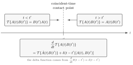
The time-ordered product is piecewise defined. As crosses , the operator order jumps from to . Differentiating this jump produces the contact term .
The same idea works for more operators. For bosonic operators ,
For regulated products satisfying the same domain and differentiability assumptions, every crossing contributes an equal-time commutator. In continuum field theory, the formula presupposes a defined time-ordered product and its contact-term prescription. The time-ordering symbol therefore carries distributional information. For fermionic operators, the corresponding formula uses graded signs and graded commutators.
The free oscillator two-point function
Section titled “The free oscillator two-point function”The free harmonic oscillator obeys
It is tempting to conclude that
That conclusion is wrong. It forgets that the differential operator acts on the time-ordering step functions.
Define
The first derivative gives
At equal time, , so the contact term vanishes:
Differentiate once more:
Now the commutator is not zero. Since and , we have
Using the equation of motion , we get
Therefore
This is the key result. The time-ordered two-point function is not an ordinary solution of the homogeneous oscillator equation. It is a Green function for the oscillator operator , with a delta-function source fixed by the canonical commutator.
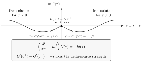
Away from , the time-ordered oscillator correlator solves the free equation. At , the derivative of the time-ordering step functions produces a delta-function source. The source strength is fixed by .
This calculation is the operator version of the inverse-kernel relation used later in the path integral. With , it is that obeys ; the raw correlator obeys . The operator derivation also identifies the source: it comes from equal-time quantization and differentiation of the ordering step functions.
Momentum-space inversion and its ambiguity
Section titled “Momentum-space inversion and its ambiguity”Since only depends on the time difference, write
Then
The Green-function equation becomes
so formally
The word “formally” matters. The expression has poles at , so the inverse is not fully specified until we say how those poles are treated. Equivalently, the differential equation determines only up to a solution of the homogeneous equation:
In Fourier language one may add distributions supported at the poles:
The equation of motion alone cannot determine and . The vacuum expectation value and the time-ordering prescription determine them. This is exactly the ambiguity that the prescription resolves.
For now, keep the lesson separate from the prescription: a propagator is an inverse only after a boundary condition has been chosen. Retarded, advanced, and Feynman Green functions invert the same differential operator but impose different boundary conditions.
Determining the oscillator propagator from modes
Section titled “Determining the oscillator propagator from modes”The oscillator mode expansion is
For ,
Only the contraction contributes. For , time ordering reverses the operators:
Thus
or, equivalently,
This expression makes the physical boundary condition visible. Positive-frequency modes propagate from the earlier insertion to the later insertion. The time-ordered product arranges the two possible orderings so that the vacuum state is used consistently.
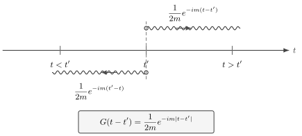
The oscillator time-ordered correlator is built from two homogeneous pieces. For , the factor is . For , time ordering gives . The discontinuity of the first derivative at supplies the delta-function source.
One can check directly that this function satisfies the Green-function equation. For , it is a sum of free oscillations, so
At , the first derivative jumps:
Therefore
which is precisely the coefficient of in . Hence
The next page rewrites this same statement as a contour prescription in the complex plane.
From the oscillator to a scalar field
Section titled “From the oscillator to a scalar field”For a free real scalar field, the equal-time canonical commutator is
The free equation of motion is
Define the time-ordered two-point function
Repeating the oscillator derivation gives
The spatial delta function enters from the equal-time commutator, while the time delta function enters from differentiating the step function in the time-ordered product.
In momentum space this becomes the formal inverse
again with the warning that the poles require a prescription. The numerator is not an arbitrary decoration: it is the same that appeared in the contact term from . The fully specified Feynman propagator is
where denotes the Feynman boundary value, developed in the next page. At finite the inverse equation belongs to the correspondingly deformed kernel.
The site’s delta-normalized Feynman inverse is a distinct object:
Thus the oscillator’s local name translates to the field correlator , not to the inverse . The Library’s time ordering and Feynman boundary value develops this normalization and its boundary conditions. The contact derivation is also given in Schwartz 2014, § 14.7.1, pp. 273–274.
Interactions and equations inside correlators
Section titled “Interactions and equations inside correlators”Now include a quartic interaction for a single time-dependent variable,
The classical equation of motion is
For the quantized anharmonic oscillator, with its Hamiltonian and a state in the required operator domains, the Heisenberg equation holds as an operator identity. Applying outside an ordered two-point function additionally differentiates the step functions:
For a bare scalar field with interaction , retain a compatible regulator, the canonical field normalization, and the same vacuum boundary prescription. In the following continuum notation, the finite-regulator version uses its regulated kinetic operator and identity kernel in place of and , and means the regulated composite insertion. The corresponding identity is
The hat means that the factor is omitted. The wave operator on the first line acts on the whole ordered correlator, not on an already ordered equation-of-motion operator. For a free field, these operations are explicitly different:
This distinction also matters in the path integral, whose derivative insertions can be denoted by a covariant prescription. It must not be identified with ordinary after using an operator equation. Schwartz 2014, § 14.7.2, p. 275 explains the distinction; lesson 17 derives the corresponding regulated source identity.
This identity is also the first glimpse of perturbation theory in correlator language. The free kinetic operator acting on an -point function produces a delta source plus a higher correlator. For , the two-point equation contains a four-field expectation value with three fields at the same point. The hierarchy is exact at the fixed compatible regulator but not closed. A continuum renormalized identity requires a specified field normalization, a renormalized composite operator , its possible mixing, and the corresponding local contact terms; the bare coincident formula cannot simply be copied unchanged. The regulated Schwinger–Dyson hierarchy makes this qualification explicit. Perturbation theory solves it order by order by expanding in and evaluating free time-ordered products with Wick’s theorem.
Summary
Section titled “Summary”Time ordering is a distributional operation. It is built from step functions, and derivatives of those step functions produce delta functions when operator times coincide. These delta functions are contact terms. They are fixed by equal-time commutation relations and cannot be dropped without destroying the Green-function equation.
For the harmonic oscillator,
obeys
For the scalar field, the same logic gives
Thus the raw propagator is times the inverse of the free equation-of-motion operator: is delta normalized. Its boundary conditions are fixed by the time-ordered vacuum expectation value. The differential equation alone leaves homogeneous solutions undetermined; the Feynman prescription, developed next, fixes that ambiguity.
Common pitfalls
Section titled “Common pitfalls”A common mistake is to move derivatives through the time-ordering symbol as if were an ordinary algebraic bracket. It is not. The step functions inside are distributions, and their derivatives produce delta functions.
Another common mistake is to confuse ordering a zero operator with differentiating an ordered product. The free operator equation remains zero when inserted inside ordinary time ordering. The contact arises when the wave operator acts outside that ordering, differentiating its step functions.
A third trap is to identify as a complete propagator. It is only a formal inverse. The poles require a prescription, and different prescriptions correspond to different Green functions.
Finally, keep track of the Lorentzian factor. Here the oscillator correlator obeys , so its delta-normalized inverse is . For the field, the corresponding names are and .
Exercises
Section titled “Exercises”Exercise 1: differentiating a time-ordered product
Section titled “Exercise 1: differentiating a time-ordered product”Let and be bosonic operators. Starting from the step-function definition of time ordering, prove
Solution
By definition,
Differentiate:
Since , the delta-function terms combine to
The remaining terms are exactly
Therefore
Exercise 2: oscillator propagator as a Green function
Section titled “Exercise 2: oscillator propagator as a Green function”For the harmonic oscillator with
compute and verify explicitly that
Solution
For ,
Only the term survives, so
For ,
Thus
For , this is a free oscillator solution, so . The first derivative is
Therefore
A function whose first derivative jumps by has a second derivative containing . Hence
Exercise 3: scalar-field contact term
Section titled “Exercise 3: scalar-field contact term”For a free scalar field with
show that
Solution
Let
The spatial derivatives do not act on the time-ordering step functions, so the only contact term comes from the two time derivatives. First,
because . Differentiating again gives
At equal time,
Thus the contact term is
Using the free equation of motion inside the non-contact part, we obtain
References
Section titled “References”- Schwartz, Matthew D. Quantum Field Theory and the Standard Model. Cambridge University Press, 2014, § 14.7, pp. 273–275. Publisher DOI.
Further reading
Section titled “Further reading”- Coleman, Sidney. Lectures of Sidney Coleman on Quantum Field Theory. Edited by Bryan Gin-ge Chen, David Derbes, David Griffiths, Brian Hill, Richard Sohn, and Yuan-Sen Ting. World Scientific, 2019. DOI. Time ordering, perturbative expansion, and Green functions.
- Srednicki, Mark. Quantum Field Theory. Cambridge University Press, 2007. DOI. Propagators, Schwinger–Dyson identities, and Ward identities.
- Weinberg, Steven. The Quantum Theory of Fields, Volume I: Foundations. Cambridge University Press, 1995. DOI. Operator derivations of Feynman rules and the canonical formalism.