

Compact Gauge Fields, Higgsing, Solitons, and Topological Defects
A gauge-field Lagrangian specifies local dynamics; the gauge group and allowed global configurations supply additional physical information. For a compact connection, holonomies are phases and charge labels are integers. Higgs fields then connect this global information to observable masses and magnetic flux. The resulting defects illustrate three separate questions: which boundary sectors exist, whether a configuration has finite energy, and whether the field equations admit a stable solution in that sector.
This lesson develops those distinctions through the Abelian Higgs vortex, an adjoint Higgs field, the scalar kink and the smooth magnetic monopole. The masses and soliton profiles below are classical or tree-level statements. Euclidean actions are identified where used; statements about topology alone do not establish a quantum phase or a monopole plasma. The preceding lesson supplies the compact-angle and vortex background.
Compact U(1) connections and holonomy
Section titled “Compact U(1) connections and holonomy”Write a local Euclidean Maxwell action in connection normalization as
The canonical field is , with covariant derivative for unit charge. The connection component has inverse-length dimension; its integral along a path is dimensionless. It is the integrated holonomy angle, not a continuum field component at a point, that is periodic.
For an oriented lattice link from to , let denote a real representative of that angle. The backward transporter in a hopping term is
Under and
the hopping term is invariant. Since and are the same group element, a character is single-valued precisely when
This normalization chooses the primitive character of the specified group. It need not be the charge of a dynamical particle: a theory can contain only charge-2 and charge-3 matter while allowing a charge-1 external Wilson probe. Specifying only the light matter does not fix all allowed probes or the global theory. This distinction is explicit in Aharony, Seiberg and Tachikawa 2013, §1.1, p. 2.
Curvature and compact monopole sectors
Section titled “Curvature and compact monopole sectors”A compact connection does not make every continuum flux identical modulo . On a closed two-surface, the first Chern number is
For example, north and south potentials on a sphere can be
They have the same curvature
Every integer gives , but the bundles and their Chern numbers remain distinct. The transition function, rather than a single potential over the whole sphere, carries the global information; see Tong 2018, §§1.1.1–1.1.2, pp. 4–8, PDF. A smooth compact connection still obeys locally. A magnetic insertion changes the domain or permitted configurations; it is not a failure of that local identity for smooth fields.
The distinction is especially concrete in a compact lattice theory. Choose real link representatives and decompose the oriented plaquette curl as
The unwrapped curls telescope around a cube . Their principal values need not:
All sums use the outward boundary orientation. In a compact Wilson lattice ensemble with action proportional to , the integers identify allowed magnetic events. In three Euclidean dimensions, a coarse description outside their regulated cores has
These are instanton events in dimensions. A continuum Maxwell action alone does not supply their core weights or prove that they proliferate. Matter, symmetries and additional action terms can restrict the allowed operators or change their effects. The next lesson treats the monopole-gas dynamics; here compactness establishes the possible global data, not the resulting phase.
Higgs mechanism and vortex flux
Section titled “Higgs mechanism and vortex flux”Consider a canonical Abelian gauge field and a charged scalar with Euclidean Lagrangian
Take and a stable radial minimum at , with positive radial mass squared. Where , write
Then
The invariant combination therefore has a quadratic mass term in local unitary gauge, giving
The calculation reorganizes physical excitations; it does not turn gauge redundancy into a spontaneously broken physical symmetry. It is local where the scalar is nonzero and cannot globally erase the winding around a vortex core. The massive-vector construction is developed in Coleman 1985, ch. 5, §2.4, pp. 122–123, Eqs. (2.37)–(2.39).
The angular finite-energy condition
Section titled “The angular finite-energy condition”Use two spatial dimensions, or the transverse plane of a straight vortex whose energy is measured per unit length. In a regular asymptotic gauge, suppose
Let be the physical angular component. For a profile whose amplitude has reached its vacuum value, the leading angular energy outside a core of radius is
Assume regular asymptotics in which the bracket has a continuous uniform limit in angle. If that limit is nonzero on any angular interval, the radial integral diverges logarithmically. Thus finite energy requires the limit to vanish. A sufficient asymptotic premise for the following contour argument is
The second statement also uses the stated nonzero vacuum amplitude and asymptotic phase with its angular derivative. Merely would be too weak: taking leaves a derivative, yet gives out to radius .
With a regular core, Stokes’ theorem and the contour limit now give
The angular cancellation and winding argument are the content of Coleman 1985, ch. 6, §§3.3–3.4, pp. 202–203 and 205–206; the sign here follows directly from . These boundary conditions are necessary data, not an existence proof for an arbitrary profile. For an actual vortex solution with positive vector and radial masses, the magnetic field and deviations of the scalar magnitude have screened tails controlled by the coupled massive-field equations. The asymptotic potential can still contain the pure-gauge term .
Adjoint Higgs field and the residual photon
Section titled “Adjoint Higgs field and the residual photon”For an gauge field, take and
Expanding the canonical scalar kinetic term gives
Thus two vector bosons have tree-level mass , while is the massless photon of the residual circle subgroup. Equivalently, a generator is unbroken when it annihilates the chosen Higgs vector. The canonical kinetic term and that criterion appear in Coleman 1985, ch. 5, §2.5, p. 126, Eqs. (2.52) and (2.54).
This local mass calculation also holds for adjoint fields with global group . Their global theories differ, however: permits a fundamental Wilson probe, while does not. This affects the interpretation of magnetic charge below. In dimensions an allowed monopole ensemble can also change the tree-level photon conclusion; the mass matrix alone does not decide that nonperturbative question.
The kink and its translation mode
Section titled “The kink and its translation mode”Consider a real scalar in one spatial dimension with
Fix the boundary values and . A finite-energy static solution obeys . Multiplication by and the vacuum boundary data give the first integral
For the increasing solution, integrating yields
The free parameter is the center. The first integral also gives its energy:
This is the standard kink construction of Coleman 1985, ch. 6, §2.1, pp. 188–191. The canonical kink treatment writes the potential with a factor ; its quartic coupling is four times the used here.
A normalizable zero eigenfunction
Section titled “A normalizable zero eigenfunction”A small Lorentzian fluctuation has linearized equation , where
Take the self-adjoint operator on with its usual domain. Integration by parts then has vanishing boundary terms. The factorization proves nonnegativity in this physical fluctuation problem, so there is no negative mode at linear order in the fixed endpoint sector.
Differentiating the classical equation gives . Its normalized eigenfunction is
It is localized around the kink center, although the kink itself tends to nonzero vacua. Since , it represents an infinitesimal translation. The differentiated equation and the zero mode’s role in linear stability are discussed in Coleman 1985, ch. 6, §2.2, pp. 191–192.
The upper curve below approaches the two vacua, while the lower curve peaks where translating the center changes the field most. To compare them on the dimensionless coordinate, define
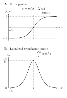
The exact classical kink (upper panel) and its dimensionless translation mode (lower panel), with . The displayed interval is ; normalization is on the whole line. At the finite endpoints, the upper curve has not reached either vacuum and the lower curve remains positive.
A continuous family of solutions similarly supplies a formal zero variation, but it is a collective coordinate only when the variation lies in the allowed normalizable domain and respects boundary and gauge conditions. A uniform phase change throughout an infinite nonzero condensate is not a localized mode. Conversely, not every zero eigenvalue in every theory must originate from a symmetry. The kink argument establishes this particular classical translation mode, not a general quantum symmetry-breaking theorem.
Defects and boundary topology
Section titled “Defects and boundary topology”Suppose that away from a core the order parameter approaches a vacuum manifold . A defect of codimension can be surrounded by a transverse linking sphere, giving
Disconnected vacuum components permit walls; describes vortex winding; and describes monopole-type boundary maps. For walls, is a set of connected components, not in general a group. A wall’s two endpoint components carry more information than merely declaring the target disconnected.
For the scalar kink, one convenient oriented label is
The kink and antikink have and . The value does not distinguish the two homogeneous vacua, so the endpoint pair should be retained when specifying the sector.
Such maps classify admissible boundary data under the chosen equivalences; they do not by themselves guarantee finite energy, a field-equation solution or dynamical stability. A gauged vacuum also requires specifying the gauge group and allowed boundary gauge transformations. The finite-energy boundary treatment separates these questions.
Global and gauged monopoles
Section titled “Global and gauged monopoles”Why a global hedgehog has divergent energy
Section titled “Why a global hedgehog has divergent energy”For a three-component global scalar in three spatial dimensions, take the asymptotic hedgehog . Its derivatives are
The leading exterior gradient energy is therefore
The nontrivial boundary map is meaningful, but the isolated global hedgehog is not a finite-energy particle in infinite volume. Its derivative tends pointwise to zero, providing another warning that decay without an integrability estimate is insufficient.
A smooth core and a Coulomb magnetic tail
Section titled “A smooth core and a Coulomb magnetic tail”For the smooth monopole, take the canonical Yang–Mills/adjoint-Higgs model with scalar kinetic term and potential
Fix at infinity, including in the zero-potential limit. Use the covariant derivative above and
With outward spatial orientation, the positive Higgs hedgehog has ansatz
Smooth solutions have , , with and near the origin; asymptotically and . The field equations determine the profiles. In particular,
so the gauge field cancels the unscreened angular scalar gradient as . It does not screen the residual photon. Directly projecting the magnetic field along the asymptotic Higgs direction gives
Here on the large sphere. The minus sign follows from the displayed covariant derivative, hedgehog and spatial orientation. The flux magnitude is ; reversing the Higgs orientation reverses the signed projection. The canonical monopole derivation gives the gauge-invariant Abelian field and the sign calculation, consistent with Prasad and Sommerfield 1975, pp. 761–762, Eqs. (20)–(21).
The remaining magnetic field falls as . Its exterior energy is finite because . Thus a smooth monopole can have a finite core and finite total energy while retaining a long-range photon field. This differs from the magnetic screening of a fully Higgsed Abelian vortex.
The global group fixes the charge interpretation
Section titled “The global group fixes the charge interpretation”For , a fundamental Wilson probe has electric charge magnitude under the residual subgroup. The smooth monopole pairs with it to give one Dirac unit in magnitude: . The charged adjoint vectors have charge magnitude .
For global group the fundamental probe is absent. The same local adjoint solution still has flux magnitude . Smooth extension through the core imposes a stronger condition than Dirac quantization for an arbitrary singular insertion. The fibration , with , gives
For , the map reduces winding modulo two. A residual bundle extending to a smooth monopole therefore has even circle winding. Its smallest nonzero flux magnitude is , even though charge- Dirac quantization permits the singular magnitude .
The choice of genuine singular lines contains further information: the theory conventionally called permits a minimal pure magnetic line, whereas has a different, dyonic minimal line. See Aharony, Seiberg and Tachikawa 2013, §1.2, pp. 4–5. Neither possibility constructs a smooth monopole of half the usual flux. Identical local Lie-algebra equations are insufficient to identify global gauge theories.
Textures and scale stability
Section titled “Textures and scale stability”A smooth texture with one fixed vacuum at spatial infinity is a map from compactified whole space, rather than from a sphere linking a core. In three spatial dimensions,
For , its degree lies in . This topology still does not fix a stable size.
To see the dynamical issue, take an admissible localized profile of finite energy and vary its physical size by . A positive two-derivative energy and a positive four-derivative energy scale in spatial dimensions as
In , a two-derivative texture lowers its energy by shrinking. A Skyrme-type four-derivative term can oppose this collapse:
The minimum is along this scaling family. It does not prove the full field equations or stability under every deformation. In , a two-derivative sigma model is scale invariant at this level; scaling alone neither excludes a lump nor selects its size. A scalar potential adds an term and changes the argument, as it does for the one-dimensional kink.
Derrick’s canonical scalar theorem has specific finite-energy and field-space hypotheses; its proof is in Coleman 1985, ch. 6, §2.4, pp. 194–195. It cannot be transferred unchanged to constrained sigma models or to the infrared-divergent global hedgehog. The scaling and stability treatment explains the admissible variations and the distinction between a virial condition and stability.
Wilson probes and long-distance dynamics
Section titled “Wilson probes and long-distance dynamics”A forward Abelian transporter along is
It transforms by , so is gauge invariant. This agrees with the backward link used in hopping; the path orientations are opposite. An external Euclidean worldline has interaction , giving exactly this insertion in . For nonzero , that probe alone determines the line integral only modulo .
With canonical non-Abelian fields and Hermitian generators, the corresponding transporter contains the coupling:
Tracing a closed transporter gives a Wilson loop. Its expectation value probes dynamics in addition to compactness and charge labels. For a long rectangular loop of separation and Euclidean time , a static-source channel has after the chosen source self-energy subtraction. A linear potential yields an area contribution. A Coulomb regime has a dimension-dependent potential as well as ultraviolet perimeter terms; it need not be a pure perimeter law. Dynamical screening and string breaking also depend on the allowed charges. The next lesson develops the conditions for a monopole plasma and Wilson-loop confinement.
Common pitfalls
Section titled “Common pitfalls”Inferring the global theory from the Maxwell term. The local quadratic action does not specify the charge lattice, allowed bundles or magnetic insertions. Exponentiated holonomy can lose information that an integer flux sector retains.
Replacing finite energy by pointwise decay. Both a global vortex and a global hedgehog have gradients that tend to zero, but their integrated energies diverge. Check the radial energy integral or state an asymptotic condition strong enough for the desired contour limit.
Promoting topology or one variational minimum to stability. A nontrivial sector does not solve the field equations. A minimum under rescaling does not test all fluctuation directions, and a formal zero variation is not necessarily a normalizable mode.
Exercises
Section titled “Exercises”Compactness and integer charge labels
Section titled “Compactness and integer charge labels”Let be a compact lattice gauge field with . A charged hopping term is
Show that is an integer in units of the primitive character, whether or not a particle of unit charge is dynamical.
Solution
The link angle and describe the same compact gauge field. Therefore the hopping factor must be single-valued:
This requires
Thus
The primitive character defines the unit; it is not inferred from the smallest charge among the dynamical fields. For integer charges with , the ratio is rational.
The adjoint-Higgs mass matrix
Section titled “The adjoint-Higgs mass matrix”Consider an gauge theory with an adjoint scalar and covariant derivative
For the vacuum , determine which gauge fields acquire a mass from .
Solution
In the chosen vacuum, , so
The components are
and
Therefore
The fields and , or equivalently , have tree-level mass . The field remains massless at tree level and is the gauge field of the unbroken .
The kink translation zero mode
Section titled “The kink translation zero mode”For a static kink satisfying
show that is a zero mode of the quadratic fluctuation operator
Solution
Differentiate the classical equation with respect to :
Rearranging gives
Thus
The zero mode exists because translating the kink center changes the solution but not its energy.
Infrared energy of a global monopole
Section titled “Infrared energy of a global monopole”Estimate the large-distance energy of a global monopole in three spatial dimensions with
and energy density .
Solution
At large , the field changes only angularly. A unit vector on the sphere has angular derivatives of order , so
The gradient energy out to radius is therefore
Hence
The energy grows linearly with system size. A global monopole is topologically meaningful but not a finite-energy particle in infinite volume.
Magnetic flux of an Abelian Higgs vortex
Section titled “Magnetic flux of an Abelian Higgs vortex”In the Abelian Higgs model, suppose that far from a regular vortex core
Take this asymptotic form together with its angular derivative, uniformly on large circles. Use the stronger condition uniformly in angle to derive flux quantization. Explain why alone would not suffice.
Solution
With , the physical angular derivative has asymptotic form
The nonzero limiting amplitude and the stated uniform condition therefore give
Integrating on a circle of radius and taking the limit is now justified:
By Stokes’ theorem for the regular core,
If instead and , the derivative falls as and hence tends to zero, but the angular energy diverges logarithmically. Pointwise decay alone cannot be integrated around circles whose length grows without bound.
References
Section titled “References”- Aharony, Ofer, Nathan Seiberg and Yuji Tachikawa. “Reading between the lines of four-dimensional gauge theories.” Journal of High Energy Physics 08 (2013), 115. DOI; Open PDF, arXiv v5.
- Coleman, Sidney. Aspects of Symmetry: Selected Erice Lectures. Cambridge University Press, 1985, chapters 5–6. DOI.
- Prasad, M. K., and C. M. Sommerfield. “Exact Classical Solution for the ’t Hooft Monopole and the Julia–Zee Dyon.” Physical Review Letters 35 (1975), 760–762. DOI.
- Tong, David. Gauge Theory. University of Cambridge lecture notes, 2018, chapter 1. Open PDF.