

Scalar Propagators and One-Loop φ⁴ Theory
The previous page developed the standard one-loop tools: Wick rotation, Feynman parameters, Schwinger parameters, and the logarithmic scalar bubble. We now put those tools to work in the simplest relativistic field theory with an interacting coupling: real scalar theory in four spacetime dimensions.
There are two lessons. First, the scalar propagator packages the oscillator physics of each momentum mode. The prescription selects vacuum time ordering; homogeneous stationary occupied states add on-shell terms whose high-momentum behavior must also be specified. Second, the one-loop vacuum correction to the four-point vertex is logarithmically ultraviolet sensitive. Its divergent part is independent of the external momenta, so it is absorbed by the same local operator that was already present in the Lagrangian.
The key calculation is
for each of the three four-point channels. Here denotes the external momentum or mass scale that cuts off the infrared end of the logarithm. This is the first appearance of the coefficient that the renormalization group will organize and resum.
Required background. Euclidean Loop Integrals and Feynman Parameters supplies the bubble integral and its logarithmic coefficient. Scalar propagators, ordered correlators, and sources supplies the free-vacuum distribution and pole prescription used below.
Helpful background. Källén–Lehmann representation explains how the free pole generalizes to stable-particle poles and multiparticle continua in an interacting vacuum. Thermal propagators and spectral representations supplies a familiar admissible occupation distribution. The occupied-state two-point function and the vacuum loop calculation below are distinct applications.
Scalar modes and the Feynman propagator
Section titled “Scalar modes and the Feynman propagator”A free real scalar field is an infinite collection of harmonic oscillators, one for each spatial momentum. On this page
so its momentum-space representation includes the numerator . For a single oscillator with frequency , the time-ordered two-point function in the vacuum is
For a field mode with momentum , the frequency is
The fixed- propagator is therefore
The prescription specifies where the poles sit:
For , the factor damps the large semicircle in the lower half-plane, so the contour encloses the positive-energy pole. For , the contour closes above and encloses the negative-energy pole. This is the frequency-space origin of the absolute value .
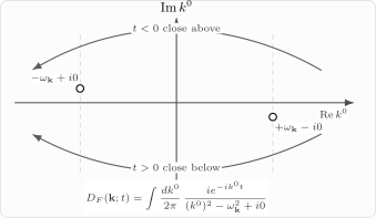
The Feynman prescription places the positive-energy pole below the real axis and the negative-energy pole above it. Closing the contour below for and above for gives .
Fourier transforming the spatial momentum gives the vacuum scalar propagator in mixed form:
This formula is often more physically transparent than the fully covariant one: each momentum mode propagates like an oscillator with frequency , and the vacuum time ordering is encoded by .
Propagators in occupied states
Section titled “Propagators in occupied states”For a free mode, the vacuum is the state with occupation number in the particle basis selected by positive frequency. If instead a single oscillator is in a number eigenstate , then
and
The time-ordered propagator becomes
The first term is the vacuum-like propagation of a quantum inserted into the state. The second term is possible because the state already contains quanta that can be removed and later replaced. In frequency space,
Equivalently,
The difference is on shell, but this does not bound the spatial momentum. For a centered, homogeneous stationary free-field state with no anomalous correlations and an even occupation function , the corresponding formula is
Without the evenness assumption the positive- and negative-frequency pieces involve and separately. Squeezed states can also have anomalous correlations, so a general state is not specified by these occupation numbers alone. The number-state calculation above determines a two-point function; it does not assert Gaussian Wick factorization of all higher correlators. That additional property holds for quasifree states, including the free thermal state.
To retain the vacuum short-distance singularity, require a suitable high-momentum falloff. In this free-field setting a useful sufficient condition is that the state-vacuum two-point difference is smooth. For example, a sufficiently regular occupation with all momentum moments integrable has this property, subject also to infrared control. The thermal distribution decreases exponentially in the ultraviolet and selects the bath’s rest frame. The precise general condition is described in Hadamard states: for the same free-field commutator, two Hadamard states have a smooth two-point difference Sanders 2010, Lemma 2.9, preprint p. 6 (PDF). Thus the same local singular subtraction can be used for their Wick observables; their finite state-dependent expectations can differ.
A simple counterexample shows why the condition matters. For a massless field in three spatial dimensions, a constant occupation gives
This state has an additional ultraviolet singularity despite the on-shell support. By contrast, gives the finite limit for . Neither example changes the vacuum bubble calculation below. State-independent vacuum counterterms are not justified merely by labeling a medium term “on shell.”
Vacuum spectral structure
Section titled “Vacuum spectral structure”The single free-particle pole is the simplest possible vacuum spectrum. In an interacting Poincaré-invariant vacuum with (or after subtracting the disconnected one-point contribution), positivity and completeness organize the exact two-point function as
A stable one-particle state contributes , while multiparticle states contribute a continuum beginning at the relevant threshold. The same Feynman boundary prescription accompanies every spectral mass.
This vacuum spectral density should not be confused with the extra on-shell term in . The former describes which invariant-mass states the field can create from the vacuum; the latter describes real quanta already occupying a chosen state and generally selects a preferred frame.
Short-distance behavior of the free scalar field
Section titled “Short-distance behavior of the free scalar field”At equal time and at distances much shorter than the Compton wavelength , the mass is negligible. The vacuum two-point function becomes
Using spherical coordinates around , one has
so
With the usual convergence factor, . Hence
The same result is obtained from the Euclidean propagator,
because for :
This singularity is the coordinate-space statement that a scalar field in four dimensions has engineering dimension one:
It also explains why is marginal by power counting in four dimensions. The product of two propagators behaves as
and the four-dimensional volume element is . Thus a short-distance loop integral contains
a logarithm. The momentum-space calculation below is the same physics written in the language of Feynman diagrams.
φ⁴ theory and the one-loop vertex
Section titled “φ⁴ theory and the one-loop vertex”Consider Euclidean real scalar theory in four dimensions,
with ultraviolet cutoff . The Euclidean propagator is
To fix the sign once and for all, define as the coefficient of in the Euclidean 1PI effective action . Thus at tree level. We first isolate the positive integral multiplying one bubble channel; its symmetry factor is :
There are three ways to pair four external legs into a bubble channel: , , and . Therefore the total one-loop logarithmic weight is three times the channel answer.
The sign follows directly from the one-loop effective action. With ,
Four derivatives of the last term produce the three pairings and give times the bubble integral in each channel. The factor and the minus sign therefore have different origins: the former is the bubble symmetry factor, while the latter is the quadratic term in the logarithm.
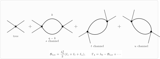
The positive bubble weight is the sum of the , , and channels, each with symmetry factor . For defined as the Euclidean effective-action coefficient, this total weight is subtracted from the tree coupling.
For the ultraviolet logarithm, assume all external momenta and the mass are of order , with
Then
and the leading logarithmic region gives
Using
we get
Thus the logarithmic contribution from all three channels is
In the 1PI effective-action convention just defined, the low-energy four-point coupling has the form
If one instead calls the Euclidean diagrammatic vertex factor itself the vertex, it is and every displayed overall sign reverses. The definition above matches the running coupling on the following lessons; within that definition the minus sign is not optional. The next page turns this coefficient into a differential RG equation.
Why the divergence is local
Section titled “Why the divergence is local”The leading ultraviolet term does not depend on the external momenta. That is the decisive fact. In the hard region,
After angular integration, the terms odd in vanish. The remaining correction is at worst and is ultraviolet convergent:
which is ultraviolet finite as . The only logarithmic part is therefore independent of external momentum. In position space this says that the short-distance singularity occurs when the two interaction points collide, leaving a local four-field operator at the collision point.
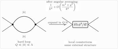
When the loop momentum is much larger than all external scales, angular averaging leaves plus UV-convergent corrections. The logarithmic part has the same local four-leg structure as the original vertex and is absorbed into a local counterterm.
This locality is the practical reason renormalization works. The ultraviolet divergence is not an arbitrary nonlocal function of the external momenta. It is proportional to an operator already present in the low-energy effective action:
Renormalization means choosing so that physical low-energy quantities are insensitive to the artificial cutoff .
A useful normalization check is obtained by differentiating only the leading logarithm. With
we find
Replacing by the running coupling inside the right-hand side gives the RG equation of page 06. This quick check is often the safest way to remember the sign: for positive , the coupling decreases toward the infrared and increases toward the ultraviolet.
Leading-log bookkeeping
Section titled “Leading-log bookkeeping”The bubble integral is not just divergent; it is the first term in a structured series. At loops, the leading logarithms in the four-point coupling have the schematic form
If but is not small, then all powers of must be kept. Terms with fewer logarithms, such as
are subleading in this approximation.
This is why constants inside logarithms do not matter at leading-log accuracy. For example,
The first term can be large; the second is an ordinary constant. In a one-loop correction, the large part scales as , while the constant part scales as . If , the logarithmic correction is of order , but the constant correction is still of order and is dropped at leading-log accuracy.
The next page will explain why the leading logarithms are not independent miracles. They are generated recursively by nested momentum regions and are summed by the renormalization-group equation.
Summary
Section titled “Summary”The scalar Feynman propagator is the oscillator propagator of each momentum mode:
The prescription chooses the vacuum time ordering by placing the positive-energy pole below and the negative-energy pole above the real axis.
An occupied state modifies the propagator by an on-shell term:
An interacting vacuum instead replaces the free spectral delta function by a positive spectral density containing stable-particle poles and multiparticle continua.
At short distances, a four-dimensional scalar propagator behaves as
Therefore a one-loop bubble in theory has a logarithmic short-distance singularity. In momentum space,
The one-loop four-point correction contains three bubble channels and a symmetry factor per channel. The universal leading logarithmic coefficient is therefore
For the coefficient of in the Euclidean 1PI effective action,
Because the logarithmic hard-loop contribution is independent of external momenta, it is local and is absorbed into the coupling.
Common pitfalls
Section titled “Common pitfalls”Do not confuse the Feynman propagator with a causal response function. The Feynman propagator is time ordered and is generally nonzero at spacelike separation. Causality is expressed by commutators or retarded functions, not by itself.
The in the occupied-state propagator is an occupation number, not a cutoff or a loop order. Its contribution is on shell and state dependent.
The factor in the one-loop vertex is two ingredients multiplied together: three channels and a symmetry factor for the two identical internal lines in each bubble.
Do not change signs midway through a calculation. On this page is the coefficient of in the Euclidean 1PI effective action, so its bubble correction is negative. The Euclidean diagrammatic vertex factor is and therefore has the opposite displayed sign.
A logarithm such as has the same leading-log content as . The difference is a finite constant and belongs to subleading accuracy.
A hard cutoff can obscure momentum-shift invariance in power-divergent terms. The logarithmic coefficient of the bubble is universal, but finite constants and power divergences are regulator dependent.
Exercises
Section titled “Exercises”Exercise 1: Vacuum contour integral
Section titled “Exercise 1: Vacuum contour integral”Evaluate
by contour integration and show that
Solution
The poles are
For , close the contour in the lower half-plane. The orientation is clockwise, so
The residue is
so
For , close in the upper half-plane. The residue at is
and the contour is counterclockwise, giving
Combining the two time orderings gives the stated result.
Exercise 2: Occupied oscillator
Section titled “Exercise 2: Occupied oscillator”For a harmonic oscillator in the number state , show that
Then show that its frequency-space form can be written as
Solution
Write
For ,
Since
we get
For , time ordering exchanges the two operators and gives the same expression with replaced by in the first exponential and by in the second. Thus
Using
and
we find
where . Therefore
Exercise 3: Short-distance scalar correlator
Section titled “Exercise 3: Short-distance scalar correlator”Show that the massless equal-time scalar propagator in four spacetime dimensions is
with , understood as a regulated distribution.
Solution
Use spherical coordinates with the polar axis along :
Then
This simplifies to
With a convergence factor ,
as . Hence
Exercise 4: Three-channel logarithm
Section titled “Exercise 4: Three-channel logarithm”Compute the leading logarithmic part of
Then use it to find the coefficient of the one-loop logarithm in the four-point vertex of real theory.
Solution
In four Euclidean dimensions,
Therefore
One bubble channel has symmetry factor , so its logarithmic weight is
There are three channels. Thus the total one-loop logarithmic weight is
Equivalently,
In the effective-action convention used on this page, the signed result is
Equivalently, the standard Euclidean diagrammatic vertex factor receives the opposite sign.
Exercise 5: Leading-log accuracy
Section titled “Exercise 5: Leading-log accuracy”Suppose a one-loop calculation gives
instead of
Explain why the difference is subleading in the leading-log approximation when but is order one.
Solution
The two logarithms differ by a constant:
Thus the difference in the one-loop correction is
In the leading-log regime,
so
The logarithmic one-loop correction is therefore parametrically of order , while the constant correction is of order . It is smaller by one power of and is not part of leading-log accuracy.
Exercise 6: One-loop beta function
Section titled “Exercise 6: One-loop beta function”Starting from the one-loop leading-log result
derive the one-loop beta-function coefficient in the convention
Solution
Introduce a renormalized coupling at scale by
The one-loop relation is
Invert to the same order:
Holding the bare coupling and cutoff fixed, differentiate with respect to :
Therefore
The positive sign means the coupling grows toward higher renormalization scales.
References
Section titled “References”- Sanders, Ko. “Equivalence of the (Generalised) Hadamard and Microlocal Spectrum Condition for (Generalised) Free Fields in Curved Spacetime.” Communications in Mathematical Physics 295 (2010): 485–501. DOI. Open PDF.
Further reading
Section titled “Further reading”- Coleman, Sidney. Lectures of Sidney Coleman on Quantum Field Theory. Edited by Bryan Gin-ge Chen, David Derbes, David Griffiths, Brian Hill, Richard Sohn, and Yuan-Sen Ting. World Scientific, 2019. See the lectures on Wick diagrams, divergences, and coupling renormalization.
- Schwartz, Matthew D. Quantum Field Theory and the Standard Model. Cambridge University Press, 2014. See Chapters 6, 7, 14, 19, and 23.
- Srednicki, Mark. Quantum Field Theory. Cambridge University Press, 2007. See Sections 3, 8–10, 16, 27, and 28.
- Weinberg, Steven. The Quantum Theory of Fields. Vol. I, Foundations, Cambridge University Press, 1995, Chapters 6 and 12; Vol. II, Modern Applications, Cambridge University Press, 1996, Section 18.2.
- Zinn-Justin, Jean. Quantum Field Theory and Critical Phenomena. 5th ed., Oxford University Press, 2021. See Chapters 2 and 8–13.