

Fixed Points, Tricriticality, and Order–Disorder Variables
The previous page constructed the Wilson–Fisher fixed point as a weakly coupled infrared fixed point in dimensions. That calculation matters, but the conceptual lesson is broader: a critical point is not just a place where a mass vanishes. It is a scale-invariant theory together with a list of perturbations. Some perturbations must be tuned away to stay critical; others disappear automatically as we look at longer distances.
This page makes that logic explicit. We first review fixed points and scaling fields. Then we explain why an ordinary Ising critical point and a tricritical Ising point are different fixed points, even though both have the same symmetry. Finally we return to the lattice Ising model and introduce the two variables that will dominate the next part of the course: the order variable and the disorder variable .
The common theme is that the long-distance theory knows about operators, not microscopic details. A polynomial Landau action gives a useful coordinate system, but the true critical theory is characterized by scaling dimensions, operator products, and defect insertions.
Required background. The epsilon expansion and one-loop scaling supplies the Wilson–Fisher fixed point, the critical surface, and the distinction between relevant and irrelevant flow directions.
Helpful background. The Ising graphical expansions supplies the closed-loop expansion, while Kramers–Wannier duality explains why a high-temperature variable can become an ordered variable in the dual model.
Scaling fields near a fixed point
Section titled “Scaling fields near a fixed point”Let be a fixed-point action. A nearby action can be written schematically as
where the are local operators. The RG acts as a flow on the couplings:
A fixed point satisfies
for every . At such a point, after relevant perturbations have been tuned away and in infinite volume, the theory has no intrinsic correlation length. Correlation functions become power laws rather than exponentials. For the unitary, short-range critical systems considered later—especially in two dimensions—scale invariance is enhanced to conformal invariance under the standard assumptions, but the RG statement is enough here.
Near the fixed point, write
Linearizing the beta functions gives
Diagonalizing gives scaling fields :
The sign of determines the fate of the perturbation:
- : grows toward long distances, so the perturbation is relevant;
- : dies toward long distances, so the perturbation is irrelevant;
- : is marginal at linear order, and nonlinear terms decide whether it is marginally relevant, marginally irrelevant, or exactly marginal.
This is the cleanest meaning of universality. Microscopic Hamiltonians contain infinitely many symmetry-allowed couplings, but most of their scaling fields are irrelevant near a stable critical fixed point. Long-distance physics remembers only a small number of relevant perturbations and a small amount of discrete information: dimension, symmetry, locality, and sometimes topology.
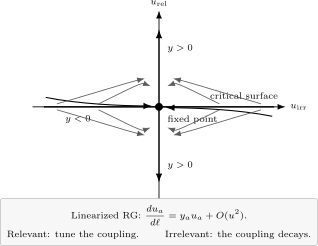
Representative linearized flow with and ; the rates are illustrative. Arrows point toward longer distances. The inward trajectories lie exactly on the critical surface , while every nonzero relevant component grows in magnitude. Nonlinear terms can bend the critical surface beyond this local linear approximation.
The set of theories that flow into the fixed point is the critical surface or stable manifold. Within a specified symmetry sector, its codimension is the number of independent relevant scaling fields that must be tuned. For the ordinary Ising universality class, if the magnetic field is forbidden by the symmetry, one tunes only a temperature-like parameter. If the magnetic field is allowed, it is another relevant perturbation.
The ordinary Ising fixed point therefore has the local form
where is temperature-like, is the magnetic field, and the multiply irrelevant operators. The fields and are the continuum energy and spin operators. Their dimensions are not generally their Gaussian dimensions; they are dynamical data of the fixed point.
Gaussian power counting as a first map
Section titled “Gaussian power counting as a first map”Before the exact scaling dimensions are known, the Gaussian fixed point gives a useful first map. Consider a real scalar field with symmetry,
and Euclidean action
At the Gaussian fixed point, the kinetic term fixes the engineering dimension of the field:
The operator has Gaussian dimension
so its coupling has RG eigenvalue
For the first few even operators,
Thus the mass term is always relevant, the quartic interaction is marginal at , and the sextic interaction is marginal at .
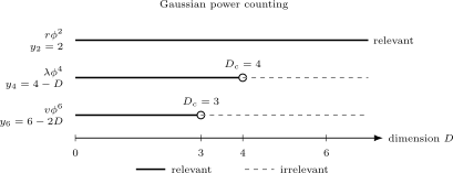
Gaussian power counting predicts the upper critical dimension of each interaction. Ordinary Ising criticality is controlled by near , while tricritical Ising behavior is controlled by near .
This is why the previous page expanded around : the quartic interaction is weakly relevant and can balance loop effects at the Wilson–Fisher fixed point. For tricriticality, the analogous expansion is around
because the stabilizing interaction is weakly relevant there.
Power counting is only the start. At an interacting fixed point, scaling dimensions are shifted by anomalous dimensions. For the spin field,
in a scalar-field normalization, so the critical two-point function behaves as
In two-dimensional Ising theory, for example,
so . Landau theory would have given . The missing quarter power is not a cosmetic correction; it is the signal of a genuinely non-Gaussian fixed point.
Dimensional estimates from the interaction
Section titled “Dimensional estimates from the interaction”The same classification can be seen without formal RG language. At a length scale , the free critical field has
The quartic interaction in a region of volume has size
Equivalently the dimensionless quartic coupling at scale is
For this goes to zero at long distances, so the Gaussian fixed point is stable. For it grows, so the Gaussian fixed point cannot describe the ordinary Ising critical theory. For it is marginal and logarithms decide the flow.
The same conclusion follows from the classical equation of motion. Schematic Euclidean theory gives
Expanding a solution as
one finds
The inverse Laplacian contributes two powers of length, while contributes three powers of the field. The relative importance of the correction is again controlled by .
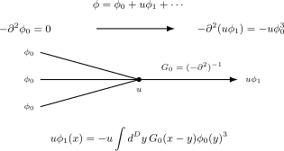
Solving the nonlinear field equation perturbatively produces tree diagrams. Loop corrections are a separate effect: they come from integrating over fluctuations around the classical solution.
Diagrams, equations of motion, and RG are just three languages for the same scale estimate.
Criticality without microscopic spin-flip symmetry
Section titled “Criticality without microscopic spin-flip symmetry”The Ising lattice model has an exact symmetry, but many physical systems in the Ising universality class do not. A liquid–gas critical point is the standard example. The coarse-grained order parameter may be taken to be a density fluctuation, and the most general local potential begins as
The field is conjugate to the order parameter. One may first shift the field so that the chosen equilibrium point is at ; its stationarity condition then removes the linear term there. Departing from that equilibrium reintroduces the ordering field . A continuous critical point also requires the curvature to vanish. If the cubic term remains nonzero, the local potential is too asymmetric to produce the Ising critical singularity; generically the system is driven toward a first-order jump. Thus, in a two-parameter family one reaches an ordinary critical point by imposing
Here and are schematic control parameters; in a magnetic system they could be replaced by other microscopic couplings. The last inequality says that the quartic term stabilizes the critical potential. In modern terminology this is ordinary Ising criticality written in asymmetric variables, not tricriticality. The infrared fixed point has an emergent spin-flip symmetry even when the microscopic variables do not.
The equations are local Landau-coordinate conditions, not invariant definitions of two separate RG eigenfields. Field shifts and analytic mixing of with change their detailed form. The invariant statement is that the two relevant Ising scaling fields—the temperature-like and ordering-field directions—must be tuned.
In an exactly Ising-symmetric model at zero magnetic field, is automatic and only the temperature-like coupling must be tuned. Without microscopic symmetry, the leading asymmetric perturbation must also be tuned away. This is the Landau version of the fixed-point rule: tune all relevant deformations not allowed at the desired critical theory.
Ordinary criticality and tricriticality
Section titled “Ordinary criticality and tricriticality”The usual Ising critical point is reached by tuning the coefficient of to zero while keeping the stabilizing quartic coupling positive. In Landau language,
At , the transition is continuous at
For , the minimum is at . For , the minima are at
and the symmetry is spontaneously broken. The order parameter vanishes continuously as
That is the mean-field exponent .
Now allow a sextic term and allow the quartic coefficient to pass through zero:
For , tuning gives the ordinary continuous transition. For , the quartic term favors a jump, and the sextic term stabilizes the potential at large . The transition becomes first order.
To find the first-order coexistence line at , set
Nonzero stationary points obey
At such a stationary point,
Using gives
Coexistence with the minimum requires with , hence
This is positive only for . Substituting back gives
The first-order line and the ordinary continuous line meet at
This meeting point is the tricritical point.
The curve above is the coexistence line, found by requiring degenerate minima. It should not be confused with the spinodal curves, where a metastable minimum disappears; those follow from the additional condition and lie elsewhere.
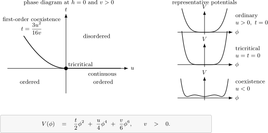
The Landau potential with contains both ordinary criticality and tricriticality. For , tuning gives a continuous Ising transition. For , the transition is first order. The two meet at , where the leading stabilizing interaction is .
Historically, “tricritical” denotes a point where a line of continuous transitions meets a line of first-order transitions. In the symmetric Landau picture, the disordered region and the two symmetry-related ordered vacua all come together there. Within the -symmetric scalar sector, RG language says that one extra relevant even perturbation must be tuned. To reach the ordinary Ising critical point at , tune . To reach the tricritical point at , tune both and .
Mean-field tricritical exponents
Section titled “Mean-field tricritical exponents”At the tricritical point the quartic term has also been tuned away, so the leading even potential is . Set and :
For , the nonzero minima obey
so
Therefore
At and , include a magnetic field:
Stationarity of the full potential gives
so and
In the symmetric phase , the susceptibility is
so
The correlation length is controlled by the mass term in the Landau–Ginzburg action,
The singular free energy below the transition is obtained by substituting the minimum. Since ,
so
Using gives
These values are mean-field exponents. Because is marginal at , three dimensions is the upper critical dimension of tricritical Ising theory, so logarithmic corrections appear there. Below three dimensions, the tricritical point is an interacting fixed point. In two dimensions it becomes a conformal field theory with a finite list of primary fields, but that belongs to the CFT part of the course.
Ordinary Ising versus tricritical Ising
Section titled “Ordinary Ising versus tricritical Ising”It is tempting to say that the tricritical theory is just ordinary Ising theory with a small quartic coupling. That is too casual. The sign and flow of the quartic perturbation decide the destination.
For the ordinary Ising transition,
At , the quartic interaction grows away from the Gaussian point and flows toward the Wilson–Fisher fixed point. Positive microscopic is not a fine tuning; it is part of the basin of attraction.
For tricritical Ising behavior,
and one must tune
The even perturbation is relevant at the tricritical point. After the temperature direction is retuned, positive sends the system toward ordinary Ising critical behavior; negative sends it toward a first-order transition.
This is the first example in the course where the same symmetry admits more than one interesting fixed point. Symmetry tells us which operators are allowed. It does not by itself tell us which fixed point controls the infrared.
Landau theory and exact criticality
Section titled “Landau theory and exact criticality”Landau theory is invaluable because it organizes phases and perturbations. It is not the exact theory of critical exponents below the upper critical dimension. The ordinary two-dimensional Ising transition is the warning sign.
For ordinary Ising mean-field theory,
The exact two-dimensional Ising fixed point instead has
with a logarithmic singularity in the specific heat. These exponents are not obtained by minimizing a polynomial potential. They are properties of the fixed point.
The right attitude is therefore:
while
The next step is to learn how to describe the operator content of the two-dimensional fixed point. For that we need a second kind of Ising variable.
Order variables
Section titled “Order variables”In the lattice Ising model, the microscopic order variable is the spin
The magnetization
is an order parameter for the broken symmetry. In the ordered phase,
In the disordered phase, the connected correlator decays exponentially:
The zero-field high-temperature expansion gives a graphical interpretation of this statement. For nearest-neighbor coupling ,
Let
Then
where is the number of bonds. Expanding the product selects a set of bonds . A spin sum survives only when every site is incident on an even number of selected bonds. Thus
For the two-point function at distinct sites , insert :
Now the surviving graphs have odd degree at and , and even degree at every other site. Therefore they contain open paths connecting and , possibly dressed by closed loops. The order-field correlator is a sum over graphs whose endpoints are order insertions.
This is the first hint that local operators are not merely functions in an action. They create allowed endpoints, twists, or singularities in the graphical expansion.
Disorder variables
Section titled “Disorder variables”The disorder variable is more subtle. It does not multiply the spin configuration by a local function of the spins. Instead it changes the couplings along a line.
Place a dual lattice site at the center of each plaquette of the square lattice. Given two dual sites and , choose a path on the dual lattice connecting them. Define signs on original-lattice bonds by
Let denote the partition function with these flipped bonds. The disorder two-point function is defined up to a local normalization by
Equivalently, the insertion flips the sign of the Ising coupling on every bond crossed by . The conventional lattice choice is , as in Kadanoff and Ceva 1971, p. 3919, Eq. (2.3), PDF. A different endpoint normalization preserves the critical powers provided is finite, positive and nonsingular near the transition; a vanishing or divergent factor need not do so.
Path deformations must preserve the boundary sector. At zero magnetic field, choose signs in a swept spin region and outside it. The change of variables changes the bond signs to and gives , provided it respects any fixed boundary spins. On a torus this requires the same path homology class modulo two: adding a noncontractible winding can change the boundary twist and the partition function. Identical endpoints alone do not determine that sector.
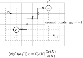
A pair of disorder variables reverses the couplings crossed by a dual-lattice line . At zero field, moving the line by a spin-region flip that preserves the boundary sector leaves the partition function unchanged. The endpoints are the local insertions; on a torus the winding sector must also be specified. This diagram shows one planar path and is schematic.
The spin-region argument is the deformation used in Kadanoff and Ceva 1971, p. 3919, PDF. The path-independence derivation in the next lesson develops it further and explains what changes when the line crosses an order insertion.
For the present page, the phase interpretation is enough. In the high-temperature phase, changing the signs of a long string of weak bonds costs little free energy, and the disorder field has long-range order. In the low-temperature phase, the insertion forces an energetically costly domain wall between its endpoints, so the disorder correlator decays. This is the opposite behavior from the spin order parameter.
The Kramers–Wannier duality relation
exchanges these two descriptions. Schematically,
while high temperature in one model becomes low temperature in the dual model. At the self-dual critical point, order and disorder are placed on equal footing.
Why both variables belong to the fixed point
Section titled “Why both variables belong to the fixed point”The order variable is local in the original spin variables, while the disorder variable is local in the dual description. At the self-dual critical point neither can be discarded: each has a power-law correlator and creates a legitimate local scaling field in its own operator algebra. Their mutual branch-cut structure and the resulting fermionic variables belong to the next two lessons, where the necessary line prescription is made explicit.
The broader lesson is that the operator content of a critical theory is richer than the polynomial action suggests. The action may begin with or , but the fixed point contains order fields, disorder fields, energy fields, descendants, and eventually a stress tensor. This operator viewpoint is the natural entrance into conformal field theory.
Summary
Section titled “Summary”A fixed point is a scale-invariant theory in coupling space. Perturbations around it are classified by RG eigenvalues . Relevant perturbations grow and must be tuned; irrelevant perturbations decay and explain universality.
The ordinary Ising critical point and the tricritical Ising point are different fixed points with the same symmetry. Ordinary Ising criticality is reached by tuning the temperature-like variable at positive quartic coupling. Tricriticality requires tuning both and the quartic coupling to zero, leaving the sextic interaction as the leading stabilizer.
Gaussian power counting gives the upper critical dimensions: for ordinary criticality and for tricriticality. Below those dimensions, interactions change the scaling dimensions.
The Ising spin is an order variable. Its correlator is represented in the high-temperature expansion by open graphs ending at the inserted spins. The disorder variable is defined by flipping couplings along a dual-lattice line. Its endpoint is a twist operator. Kramers–Wannier duality exchanges order and disorder.
Common pitfalls
Section titled “Common pitfalls”Letting symmetry choose the fixed point. Ordinary and tricritical Ising theories both have symmetry, but their relevant spectra and critical exponents differ. Symmetry determines which operators are allowed, not which fixed point controls the infrared.
Calling any small quartic coupling tricritical. The quartic perturbation is relevant at the tricritical point and must be tuned to zero. The sextic term must remain positive to stabilize the Landau potential.
Promoting mean-field exponents below the upper critical dimension. Landau theory correctly identifies phases and tuning parameters, but anomalous dimensions and critical exponents are fixed-point data. In two dimensions the exact Ising exponents differ sharply from their mean-field values.
Treating as a local polynomial in the original spins. A disorder pair is defined by modifying Boltzmann weights along a line. Its position is deformable within the fixed boundary sector, with the endpoints held fixed. On a torus, changing the winding is an additional physical choice.
The Library treatment of Critical Surfaces, Crossover, and Corrections to Scaling develops the general geometry behind tuning to ordinary and multicritical behavior. It complements this lesson’s explicit potentials and flow examples without replacing their stated approximation regimes.
Exercises
Section titled “Exercises”Exercise 1: Upper critical dimensions
Section titled “Exercise 1: Upper critical dimensions”At the Gaussian fixed point in dimensions, compute the engineering dimension of the coupling multiplying for integer :
For which dimension is marginal?
Solution
The kinetic term gives
Therefore
Since the action is dimensionless,
Thus
The coupling is marginal when
so
For , for . For , for . The excluded case has in every dimension and has no marginal dimension.
Exercise 2: The tricritical coexistence line
Section titled “Exercise 2: The tricritical coexistence line”For
show that for the first-order coexistence line between and is
in the normalization used on this page.
Solution
Let
A nonzero stationary point obeys
so
At the stationary point,
Substitute :
Coexistence with the minimum requires with :
Thus
This is positive only when . Then
Exercise 3: Mean-field tricritical exponents
Section titled “Exercise 3: Mean-field tricritical exponents”At the tricritical mean-field point , derive and .
Solution
Set first. The potential is
For , nonzero minima obey
so
Therefore
and
At and , include the magnetic field:
The equation of state is
Thus
so
Exercise 4: Open graphs from order insertions
Section titled “Exercise 4: Open graphs from order insertions”At zero field and for distinct sites , use the high-temperature expansion to show that the numerator of is a sum over graphs with odd degree at and , and even degree at every other site.
Solution
Start from
The numerator is proportional to
Expanding the product selects a set of bonds . The spin dependence of a selected graph is
At a site , the power of is the number of selected bonds incident on . The spin sum
vanishes unless is even. At distinct and , the inserted factor contributes one extra power of the spin, so the selected-bond degree must be odd there. Therefore the surviving graphs have odd degree at and and even degree elsewhere. Such graphs contain open paths from to , possibly together with closed loops. For coincident insertions, instead, and the ordinary even-degree partition-function graphs survive.
Exercise 5: Classical corrections and the quartic scale
Section titled “Exercise 5: Classical corrections and the quartic scale”For the critical classical equation
write . If a free critical configuration varying on scale has , show that
Solution
At successive orders in ,
On a configuration varying over distance , the inverse Laplacian contributes a factor of order . Therefore
Dividing by and using gives
Thus the classical perturbation is irrelevant for , relevant for , and marginal by power counting at , in agreement with the RG analysis.
References
Section titled “References”- L. P. Kadanoff and H. Ceva, “Determination of an Operator Algebra for the Two-Dimensional Ising Model,” Physical Review B 3 (1971), 3918–3939, doi:10.1103/PhysRevB.3.3918.
Further reading
Section titled “Further reading”- P. Di Francesco, P. Mathieu, and D. Sénéchal, Conformal Field Theory, Graduate Texts in Contemporary Physics, Springer, New York, 1997.
- L. D. Landau and E. M. Lifshitz, Statistical Physics, Part 1, 3rd ed., Course of Theoretical Physics, vol. 5, Butterworth–Heinemann, Oxford, 1980.
- I. D. Lawrie and S. Sarbach, “Theory of Tricritical Points,” in C. Domb and J. L. Lebowitz (eds.), Phase Transitions and Critical Phenomena, vol. 9, Academic Press, London, 1984, 1–161.
- K. G. Wilson and J. Kogut, “The Renormalization Group and the Expansion,” Physics Reports 12 (1974), 75–199, doi:10.1016/0370-1573(74)90023-4.
- J. Zinn-Justin, Quantum Field Theory and Critical Phenomena, 4th ed., International Series of Monographs on Physics, vol. 113, Oxford University Press, Oxford, 2002.