Rindler Coordinates and Green Functions

The previous page explained particle creation as a mismatch between positive-frequency modes in the past and positive-frequency modes in the future. Rindler quantization changes the question: the spacetime and state can remain stationary, but an observer confined to one accelerated wedge uses Lorentz boosts rather than inertial time translations to define energy. Positive frequency, the Hamiltonian, and the accessible algebra of observables all change.

The main object on this page is not yet the detector response or the full Unruh-effect derivation. Those come next. The goal here is to build the machinery cleanly: Rindler coordinates, the right wedge, the boost Hamiltonian, the scalar-field mode equation, and Green functions written both globally and in Rindler modes. The key surprise is already visible at the level of two-point functions:

$$\text{Minkowski vacuum restricted to one Rindler wedge} \quad\text{has thermal analyticity in Rindler time.}$$

That statement is encoded in the analytic structure of the Minkowski Wightman function. Merely changing coordinates does not create particles; thermality arises from the Minkowski state, boost evolution, and restriction to one wedge together.

Required background. Bogoliubov transformations and pair creation supplies the mode-basis logic used here, while Lorentz boosts supply the generator that becomes Rindler time evolution.

Helpful background. Wightman and related structural frameworks reviews the state-sensitive two-point functions used to diagnose thermality.

Right Rindler wedge and accelerated worldlines

Coordinates and acceleration scale

Use the global mostly-minus convention

$$ds^2=dT^2-dX^2-d\mathbf y^2,$$

where $\mathbf y$ denotes the transverse coordinates. The right Rindler wedge is

$$X>|T|.$$

Inside it, set

$$T=\rho\sinh\eta, \qquad X=\rho\cosh\eta, \qquad \rho>0, \qquad -\infty<\eta<\infty.$$

Then

$$ds^2=\rho^2d\eta^2-d\rho^2-d\mathbf y^2.$$

The coordinate $\eta$ is dimensionless boost time. Along a worldline $\rho=\rho_0$, proper time is $s=\rho_0\eta$ and proper acceleration is $1/\rho_0$. For one chosen observer it is convenient to set $\rho_0=1/a_0$ and write $\eta=a_0s$.

Quantity	Minkowski description	Right-wedge Rindler description
time translation	generated by $P^0$	generated by the boost $K_R$
observer at rest	$X=\text{constant}$	$\rho=\text{constant}$ hyperbola
proper time	$T$ for inertial rest frame	$s=\rho_0\eta$ at fixed $\rho_0$
horizon	none for inertial observer	future half-ray $U=0$, $V\geq0$; past half-ray $V=0$, $U\leq0$
vacuum adapted to time	Minkowski vacuum $\lvert0_M\rangle$	Rindler vacuum $\lvert0_R\rangle$

The two time evolutions are generated by different operators, so “positive frequency” is a different statement in the two columns.

Introduce light-cone coordinates

$$U=T-X, \qquad V=T+X.$$

The right wedge is equivalently

$$U<0, \qquad V>0.$$

In Rindler coordinates,

$$U=-\rho e^{-\eta}, \qquad V=\rho e^\eta.$$

The two null boundaries of the right wedge are the half-rays

$$U=0,\quad V\geq0 \qquad\text{(future horizon)},$$

and

$$V=0,\quad U\leq0 \qquad\text{(past horizon)}.$$

They are horizons for observers who remain at fixed $\rho$. The curves $\rho=\text{constant}$ are hyperbolae,

$$X^2-T^2=\rho^2.$$

They are the worldlines of uniformly accelerated observers. Along such a curve,

$$ds^2=\rho^2d\eta^2,$$

so the proper time $s$ is

$$s=\rho\eta.$$

The four-velocity is

$$u^\mu={dX^\mu\over ds}=(\cosh\eta,\sinh\eta),$$

and the four-acceleration is

$$a^\mu={du^\mu\over ds}={1\over\rho}(\sinh\eta,\cosh\eta).$$

Thus

$$a_\mu a^\mu=-{1\over\rho^2},$$

and the positive proper-acceleration magnitude is

$$\boxed{a_{\rm proper}={1\over\rho}.}$$

At fixed finite $\eta$, the limit $\rho\to0$ reaches the bifurcation surface $T=X=0$ rather than a generic point on a horizon. To reach the future or past horizon at nonzero null coordinate, one takes $\rho\to0$ and $\eta\to\pm\infty$ together while holding $V$ or $U$ fixed. This correlated limit matters when continuing mode functions across a horizon.

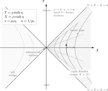
The right Rindler wedge $X>|T|$ is covered by $T=\rho\sinh\eta$, $X=\rho\cosh\eta$. Curves of constant $\rho$ are uniformly accelerated worldlines. Constant-$\eta$ slices meet at the bifurcation surface; the two null edges are the past and future horizons.

The coordinate system covers only one wedge of Minkowski space. This is already a warning: the Rindler Hamiltonian cannot be the same operator as the Minkowski Hamiltonian. Rindler time translations are Lorentz boosts,

$$\eta\mapsto\eta+c.$$

In light-cone coordinates this acts as

$$U\mapsto e^{-c}U, \qquad V\mapsto e^cV.$$

The corresponding Killing vector is

$$\partial_\eta=X\partial_T+T\partial_X.$$

On the $T=0$ half-space, the positive right-wedge boost charge is

$$\boxed{ K_R=\int_{X>0}dX\,d^{d-2}\mathbf y\;X\,T_{00}(0,X,\mathbf y). }$$

This is the operator later appearing in the reduced density matrix $\rho_R\propto e^{-2\pi K_R}$. The global Lorentz-boost generator also contains the left wedge, with the opposite future-directed time orientation there.

A Rindler observer has access only to field operators in one wedge. A constant-$\eta$ slice is a Cauchy surface for the wedge but not for all Minkowski space. This loss of access to the complementary wedge is the geometric seed of the thermal behavior that appears more explicitly on the next page.

Euclidean origin of Rindler time

Rindler coordinates are the Lorentzian continuation of ordinary polar coordinates. Start with the Euclidean $(T_E,X)$ plane and set

$$T_E=\rho\sin\theta, \qquad X=\rho\cos\theta.$$

Then

$$ds_E^2=dT_E^2+dX^2=d\rho^2+\rho^2d\theta^2.$$

Analytically continue

$$T_E=iT, \qquad \theta=i\eta.$$

This gives

$$T=\rho\sinh\eta, \qquad X=\rho\cosh\eta,$$

and therefore the Lorentzian Rindler metric

$$ds^2=\rho^2d\eta^2-d\rho^2.$$

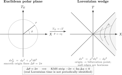
Rindler time is analytically continued polar angle. Smoothness of the Euclidean origin fixes the angular period to $2\pi$; after continuation, correlators inherit a strip of height $2\pi$ in imaginary boost time.

This Euclidean viewpoint is extremely efficient. The origin $\rho=0$ continues to the bifurcation surface of the Lorentzian horizons; it is not a physical wall or a curvature singularity. A smooth Euclidean plane requires the angular coordinate to have period $2\pi$:

$$\theta\sim\theta+2\pi.$$

After $\theta=i\eta$, Euclidean correlation functions inherit the shift

$$\eta\longrightarrow\eta-2\pi i.$$

This is an analytic continuation, not an identification of real Lorentzian time. For Wightman functions the precise thermal statement is the KMS boundary relation: the shift by $-2\pi i$ reverses operator ordering after analytic continuation through the strip. Ordinary periodicity of a denominator, by itself, is not enough.

For an observer at $\rho=\rho_0$, proper time is $s=\rho_0\eta$, so the strip has height

$$\beta_{\rm loc}=2\pi\rho_0={2\pi\over a_{\rm proper}}.$$

Thus a regular Euclidean plane selects the temperature $T_{\rm loc}=1/(2\pi\rho_0)=a_{\rm proper}/(2\pi)$. Choosing any other Euclidean angular period produces a conical singularity at the origin and therefore a different, horizon-singular state.

The scalar field in Rindler variables

Consider a real scalar field of mass $m$ in $1+1$ dimensions. The action in the global convention is

$$S={1\over2}\int d^2x\left(\partial_\mu\phi\,\partial^\mu\phi-m^2\phi^2\right).$$

In Rindler coordinates,

$$\sqrt{|g|}=\rho, \qquad g^{\eta\eta}={1\over\rho^2}, \qquad g^{\rho\rho}=-1.$$

Therefore

$$S={1\over2}\int d\eta\,d\rho\, \left[{1\over\rho}(\partial_\eta\phi)^2-\rho(\partial_\rho\phi)^2-\rho m^2\phi^2\right].$$

It is useful to introduce a dimensionless logarithmic radial coordinate using an arbitrary fixed reference length $\rho_\star>0$:

$$\rho=\rho_\star e^\xi, \qquad \xi=\log{\rho\over\rho_\star}, \qquad -\infty<\xi<\infty.$$

Then

$$ds^2=\rho_\star^2e^{2\xi}(d\eta^2-d\xi^2),$$

and the action becomes

$$\boxed{ S={1\over2}\int d\eta\,d\xi\, \left[(\partial_\eta\phi)^2-(\partial_\xi\phi)^2 -(m\rho_\star)^2e^{2\xi}\phi^2\right]. }$$

This formula explains why $\xi$ is a good coordinate for quantization in the wedge. The kinetic terms look like those of a scalar field on a line, while the mass becomes a position-dependent potential that grows exponentially as $\xi\to+\infty$. Changing $\rho_\star$ only translates the origin of $\xi$ and cannot affect physical results.

The canonical momentum conjugate to $\phi$ with respect to Rindler time $\eta$ is

$$\pi(\eta,\xi)=\partial_\eta\phi(\eta,\xi),$$

and the Rindler Hamiltonian is

$$\boxed{ H_R={1\over2}\int_{-\infty}^{\infty}d\xi\, \left[\pi^2+(\partial_\xi\phi)^2 +(m\rho_\star)^2e^{2\xi}\phi^2\right]. }$$

This is the Hamiltonian that counts Rindler energy. Up to the usual operator ordering and boundary-domain qualifications, it is the right-wedge boost charge $K_R$, not the Minkowski Hamiltonian $P^0$.

In $d$ dimensions, Fourier transform along the transverse directions:

$$\phi(\eta,\xi,\mathbf y) =e^{i\mathbf k\cdot\mathbf y}e^{-i\omega\eta}f_{\omega\mathbf k}(\xi),$$

and define

$$\kappa^2=m^2+\mathbf k^2.$$

For the radial-mode discussion below, assume $\kappa>0$. The exceptional massless transverse zero mode, $m=0$ and $\mathbf k=0$, instead obeys the free equation $f''+\omega^2f=0$ for every $\xi$; it has waves $e^{\pm i\omega\xi}$ but no large-$\rho$ barrier and is not represented by the decaying Kontorovich–Lebedev modes.

The mode equation becomes

$$\boxed{ \left[\partial_\xi^2+\omega^2 -(\kappa\rho_\star)^2e^{2\xi}\right]f_{\omega\mathbf k}(\xi)=0. }$$

Equivalently, with

$$u=\kappa\rho_\star e^\xi=\kappa\rho,$$

one gets

$$\left[u^2{d^2\over du^2}+u{d\over du}+\omega^2-u^2\right]f(u)=0.$$

The solution that decays for large $u$ is the modified Bessel function

$$\boxed{ f_{\omega\mathbf k}(\rho)\propto K_{i\omega}(\kappa\rho). }$$

Near the horizon $\rho\to0$, or $\xi\to-\infty$, the exponential potential disappears and the modes become ordinary waves in $\xi$:

$$f_{\omega\mathbf k}(\xi) \sim A_\omega e^{i\omega\xi}+A_\omega^*e^{-i\omega\xi}.$$

Far from the horizon, $\xi\to+\infty$, the potential $(\kappa\rho_\star)^2e^{2\xi}$ grows and $K_{i\omega}(\kappa\rho_\star e^\xi)$ decays exponentially.

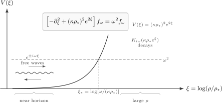
The Rindler mode equation is a one-dimensional scattering problem in $\xi=\log(\rho/\rho_\star)$. Near the horizon $\xi\to-\infty$, modes are free waves. At large $\xi$, the effective potential $V(\xi)=(\kappa\rho_\star)^2e^{2\xi}$ reflects them. The decaying radial solution is $K_{i\omega}(\kappa\rho_\star e^\xi)$.

For $\omega,\omega'>0$, the orthogonality relation behind this mode expansion is the Kontorovich–Lebedev relation

$$\int_{-\infty}^{\infty}d\xi\, K_{i\omega}(\kappa\rho_\star e^\xi) K_{i\omega'}(\kappa\rho_\star e^\xi) ={\pi^2\over 2\omega\sinh(\pi\omega)}\delta(\omega-\omega').$$

Thus a convenient normalized radial wavefunction is

$$\psi_{\omega\kappa}(\rho) ={1\over\pi}\sqrt{2\omega\sinh(\pi\omega)}\,K_{i\omega}(\kappa\rho),$$

so that

$$\int_{-\infty}^{\infty}d\xi\, \psi_{\omega\kappa}(\rho_\star e^\xi) \psi_{\omega'\kappa}(\rho_\star e^\xi) =\delta(\omega-\omega').$$

The Rindler-vacuum Green function

Expand the field in right-wedge modes,

$$\phi(\eta,\rho,\mathbf y) =\int_0^\infty d\omega\int {d^{d-2}\mathbf k\over(2\pi)^{d-2}} {1\over\sqrt{2\omega}} \left[ b_{\omega\mathbf k}\,e^{-i\omega\eta+i\mathbf k\cdot\mathbf y}\psi_{\omega\kappa}(\rho) +b_{\omega\mathbf k}^\dagger e^{i\omega\eta-i\mathbf k\cdot\mathbf y}\psi_{\omega\kappa}(\rho) \right],$$

with

$$[b_{\omega\mathbf k},b_{\omega'\mathbf k'}^\dagger] =\delta(\omega-\omega')(2\pi)^{d-2}\delta^{(d-2)}(\mathbf k-\mathbf k').$$

The right Rindler vacuum is defined by

$$b_{\omega\mathbf k}|0_R\rangle=0.$$

Its time-ordered Green function is

$$G_F^{R}(x,x')= \langle0_R|T_\eta\phi(x)\phi(x')|0_R\rangle.$$

Substituting the mode expansion gives

$$\boxed{ G_F^{R}(x,x') =\int_0^\infty d\omega\int {d^{d-2}\mathbf k\over(2\pi)^{d-2}} {\psi_{\omega\kappa}(\rho)\psi_{\omega\kappa}(\rho')\over2\omega} \,e^{i\mathbf k\cdot(\mathbf y-\mathbf y')} \,e^{-i\omega|\eta-\eta'|}. }$$

This is the direct analogue of the harmonic-oscillator Feynman function,

$${1\over2\omega}e^{-i\omega|t-t'|},$$

but now each oscillator is a Rindler mode labelled by $\omega$ and $\mathbf k$.

For $1+1$ dimensions, there is no transverse momentum and $\kappa=m$. Substituting the normalized Kontorovich–Lebedev modes gives

$$G_F^R(\eta,\rho;\eta',\rho') =\int_0^\infty d\omega\, {\sinh(\pi\omega)\over\pi^2} K_{i\omega}(m\rho)K_{i\omega}(m\rho') e^{-i\omega|\eta-\eta'|}.$$

This Green function is built from positive frequency with respect to boost time. It is the propagator of the Rindler vacuum, not the restriction of the Minkowski vacuum. The exact measure matters: dropping the factor inherited from radial-mode normalization changes the derivative jump and therefore no longer inverts the Klein–Gordon operator.

The Minkowski Green function in Rindler variables

The Minkowski vacuum is defined globally by positive frequency with respect to $T$, not by positive frequency with respect to $\eta$. Its two-point function is a function of the invariant separation. For a massless scalar in four dimensions,

$$G_M^+(X,X')= \langle0_M|\phi(X)\phi(X')|0_M\rangle ={1\over4\pi^2}\,{1\over-(T-T'-i0)^2+|\mathbf X-\mathbf X'|^2}.$$

Restrict both points to the right wedge. With

$$T=\rho\sinh\eta, \qquad X=\rho\cosh\eta,$$

the algebraic part of the invariant separation is

$$-(T-T')^2+(X-X')^2+|\mathbf y-\mathbf y'|^2 =\rho^2+\rho'^2-2\rho\rho'\cosh(\eta-\eta')+|\mathbf y-\mathbf y'|^2.$$

Within one wedge, $\eta$ is a time function: causally related events have the same ordering in $T$ and $\eta$. The Minkowski positive-frequency boundary value may therefore be written equivalently as $\Delta\eta\to\Delta\eta-i0$.

Thus

$$\boxed{ G_M^+(x,x') ={1\over4\pi^2} {1\over \rho^2+\rho'^2-2\rho\rho'\cosh(\eta-\eta'-i0)+|\mathbf y-\mathbf y'|^2 }. }$$

This formula contains the whole story in compressed form. First, it is not the Rindler-vacuum Wightman function. Second, its analytic continuation involves the identity

$$\eta-\eta'\mapsto \eta-\eta'+2\pi i,$$

because

$$\cosh(z+2\pi i)=\cosh z.$$

Naively calling this identity “periodicity” loses the boundary prescription. The function is analytic between neighboring singularity lines; its upper boundary is $G_M^+$, while its lower boundary is the oppositely ordered function $G_M^-$. The precise statement is

$$\boxed{ G_M^+(\Delta\eta-2\pi i)=G_M^-(\Delta\eta) }$$

as a relation between those boundary values. This is the KMS condition at inverse boost temperature $2\pi$.

At equal $\rho$ and equal transverse position, the expression reduces to

$$G_M^+(\Delta\eta) =-{1\over16\pi^2\rho^2} {1\over\sinh^2\left({\Delta\eta-i0\over2}\right)}.$$

If $\eta=a_0s$ at $\rho=1/a_0$, this becomes

$$G_M^+(\Delta s) =-{a_0^2\over16\pi^2} {1\over\sinh^2\left({a_0(\Delta s-i0)\over2}\right)}.$$

The imaginary proper-time period is $2\pi/a_0$. This is the analytic seed of the Unruh temperature

$$T_U={a_0\over2\pi}.$$

We will derive the detector interpretation next.

Rindler modes versus Minkowski vacuum

The difference between $|0_R\rangle$ and $|0_M\rangle$ can be seen directly in the mode expansion. The Rindler-vacuum Wightman function contains only the positive boost-frequency term

$$G_R^+(x,x') =\int_0^\infty d\omega\int {d^{d-2}\mathbf k\over(2\pi)^{d-2}} {\psi_{\omega\kappa}(\rho)\psi_{\omega\kappa}(\rho')\over2\omega} e^{i\mathbf k\cdot\Delta\mathbf y}e^{-i\omega\Delta\eta}.$$

The Minkowski Wightman function restricted to the right wedge has the thermal form

$$\boxed{ G_M^+(x,x') =\int_0^\infty d\omega\int {d^{d-2}\mathbf k\over(2\pi)^{d-2}} {\psi_{\omega\kappa}(\rho)\psi_{\omega\kappa}(\rho')\over2\omega} e^{i\mathbf k\cdot\Delta\mathbf y} \left[(1+n_\omega)e^{-i\omega\Delta\eta}+n_\omega e^{i\omega\Delta\eta}\right], }$$

where

$$n_\omega={1\over e^{2\pi\omega}-1}.$$

This is a Bose–Einstein distribution at inverse temperature

$$\beta_R=2\pi$$

with respect to dimensionless boost time. For an observer at $\rho=1/a_0$, physical proper time is $s=\eta/a_0$, so

$$\beta={2\pi\over a_0}.$$

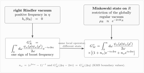
The Rindler-vacuum propagator contains only positive boost-frequency modes. The Minkowski vacuum restricted to one wedge contains both signs of boost frequency with Bose–Einstein weights $n_\omega=(e^{2\pi\omega}-1)^{-1}$.

Equivalently, tracing the pure Minkowski vacuum over the inaccessible left-wedge degrees of freedom gives

$$\boxed{ \rho_R=\operatorname{Tr}_L|0_M\rangle\langle0_M| ={e^{-2\pi K_R}\over\operatorname{Tr}_R e^{-2\pi K_R}}. }$$

In continuum QFT, the factorization and trace in this formula are regulator-dependent shorthand; the exact statement is that the Minkowski vacuum restricted to the wedge algebra is a KMS state for boost evolution. This is the same basis-mismatch structure met in the Bogoliubov discussion, but it is not dynamical pair creation by acceleration. The global state is stationary and pure; restriction to the right-wedge algebra produces the thermal state, with the left wedge providing its formal Fock-space purification.

Real-time prescriptions

It is worth separating three related Green functions. The Wightman function is ordered by neither Minkowski time nor Rindler time:

$$G^+(x,x')=\langle\phi(x)\phi(x')\rangle.$$

The Feynman function ordered by Rindler time is

$$G_F(x,x')=\theta(\eta-\eta')G^+(x,x')+\theta(\eta'-\eta)G^+(x',x).$$

To match the correlator convention on the preceding lesson, define the retarded commutator without a leading factor of $-i$:

$$D_R(x,x')=\theta(\eta-\eta')\langle[\phi(x),\phi(x')]\rangle.$$

For a perturbation $H\to H-h\phi$, the linear-response kernel is $iD_R$. Texts that define $G^R=-iD_R$ distribute these factors differently.

Inside a single wedge, ordering by $\eta$ is compatible with causal ordering for timelike-separated points, but it is not a global time ordering on all of Minkowski space. This is why the in–in language from the previous pages remains important. A detector following a fixed-$\rho$ worldline responds to Wightman functions along that worldline, not to a vacuum-to-vacuum amplitude alone.

The familiar $i0$ prescriptions are also different pieces of information. For a massless scalar in flat space,

$$G^+(X-X')={1\over4\pi^2} {1\over-(T-T'-i0)^2+|\mathbf X-\mathbf X'|^2},$$

whereas the Feynman function is obtained by time ordering. Their difference gives the commutator,

$$G^+(x,x')-G^+(x',x)=\langle[\phi(x),\phi(x')]\rangle.$$

The commutator controls causal response. The Wightman function controls what a detector clicks on. Rindler thermality is a statement about the latter.

Summary

Rindler coordinates cover the right wedge of Minkowski space:

$$T=\rho\sinh\eta, \qquad X=\rho\cosh\eta.$$

Constant-$\rho$ curves are uniformly accelerated worldlines with proper acceleration $1/\rho$. The Rindler Hamiltonian generates boosts, not Minkowski time translations. In the logarithmic coordinate $\rho=\rho_\star e^\xi$, a scalar field has Hamiltonian

$$H_R={1\over2}\int d\xi\, \left[\pi^2+(\partial_\xi\phi)^2 +(m\rho_\star)^2e^{2\xi}\phi^2\right],$$

and modes proportional to

$$K_{i\omega}(\kappa\rho).$$

The Rindler-vacuum propagator is built from positive boost-frequency modes. The Minkowski vacuum restricted to the right wedge instead obeys the KMS boundary condition at inverse boost temperature $2\pi$ and has a thermal mode expansion with

$$n_\omega={1\over e^{2\pi\omega}-1}.$$

This is the mathematical core of the Unruh effect. The next page gives its physical detector interpretation.

Common pitfalls

Do not identify the Rindler Hamiltonian with the Minkowski Hamiltonian. The former generates boosts, while the latter generates translations in $T$.

Do not say that the Rindler horizon is a curvature singularity. Flat spacetime is regular there. At finite $\eta$, $\rho\to0$ reaches only the bifurcation surface; generic horizon points require a correlated $\rho\to0$, $|\eta|\to\infty$ limit.

Do not confuse the Rindler vacuum with the Minkowski vacuum. The Rindler vacuum is singular on the horizons; the Minkowski vacuum is globally regular and appears thermal when restricted to one wedge.

Do not infer thermality from algebraic imaginary-time periodicity alone. The KMS statement includes analyticity in a strip and relates opposite operator orderings on its two boundaries. Detector response is governed by the resulting Wightman function along the detector trajectory.

Finally, a coordinate transformation does not dynamically create particles. The thermal right-wedge state results from restricting the globally regular Minkowski vacuum and evolving with the boost generator.

Exercises

Exercise 1: acceleration of a Rindler observer

For the worldline

$$T=\rho_0\sinh\eta, \qquad X=\rho_0\cosh\eta,$$

show that the proper acceleration is $1/\rho_0$.

Solution

Along the worldline,

$$ds^2=\rho_0^2d\eta^2.$$

Thus proper time is

$$s=\rho_0\eta.$$

The four-position is

$$X^\mu(s)=\left(\rho_0\sinh {s\over\rho_0},\rho_0\cosh {s\over\rho_0}\right).$$

The four-velocity is

$$u^\mu={dX^\mu\over ds} =\left(\cosh {s\over\rho_0},\sinh {s\over\rho_0}\right),$$

and the four-acceleration is

$$a^\mu={du^\mu\over ds} ={1\over\rho_0}\left(\sinh {s\over\rho_0},\cosh {s\over\rho_0}\right).$$

With metric $\eta_{\mu\nu}=\operatorname{diag}(+,-)$,

$$a_\mu a^\mu={1\over\rho_0^2}\left(\sinh^2 {s\over\rho_0}-\cosh^2 {s\over\rho_0}\right) =-{1\over\rho_0^2}.$$

Therefore

$$\sqrt{-a_\mu a^\mu}={1\over\rho_0}.$$

Exercise 2: Rindler mode equation

For a massive scalar with $m>0$, set $\rho=\rho_\star e^\xi$ and start from

$$S={1\over2}\int d\eta\,d\xi\, \left[(\partial_\eta\phi)^2-(\partial_\xi\phi)^2 -(m\rho_\star)^2e^{2\xi}\phi^2\right],$$

derive the mode equation for $\phi=e^{-i\omega\eta}f(\xi)$ and show that the decaying solution is $K_{i\omega}(m\rho_\star e^\xi)$.

Solution

The Euler–Lagrange equation is

$$\partial_\eta^2\phi-\partial_\xi^2\phi +(m\rho_\star)^2e^{2\xi}\phi=0.$$

Substitute

$$\phi=e^{-i\omega\eta}f(\xi).$$

This gives

$$-\omega^2f-f''+(m\rho_\star)^2e^{2\xi}f=0,$$

or

$$f''+\left[\omega^2-(m\rho_\star)^2e^{2\xi}\right]f=0.$$

Let

$$u=m\rho_\star e^\xi.$$

Then

$${d\over d\xi}=u{d\over du}, \qquad {d^2\over d\xi^2}=u^2{d^2\over du^2}+u{d\over du}.$$

The equation becomes

$$\left[u^2{d^2\over du^2}+u{d\over du}+\omega^2-u^2\right]f(u)=0.$$

This is the modified Bessel equation of imaginary order. A basis of solutions is $I_{i\omega}(u)$ and $I_{-i\omega}(u)$. Their particular linear combination $K_{i\omega}(u)$ cancels the growing large-$u$ behavior and decays exponentially, so the required solution is

$$f(u)=K_{i\omega}(u)=K_{i\omega}(m\rho_\star e^\xi).$$

Exercise 3: invariant separation in Rindler coordinates

For two points in the right wedge with the same transverse coordinates, prove that

$$(T-T')^2-(X-X')^2=-\rho^2-\rho'^2+2\rho\rho'\cosh(\eta-\eta').$$

Then show that the algebraic denominator is invariant under $\eta-\eta'\mapsto\eta-\eta'+2\pi i$, and explain why this identity must be supplemented by an analytic strip and boundary prescriptions to become a thermal statement.

Solution

Use

$$T=\rho\sinh\eta, \qquad X=\rho\cosh\eta.$$

Then

$$(T-T')^2-(X-X')^2 =\rho^2(\sinh^2\eta-\cosh^2\eta) +\rho'^2(\sinh^2\eta'-\cosh^2\eta')$$ $$-2\rho\rho'(\sinh\eta\sinh\eta'-\cosh\eta\cosh\eta').$$

Since

$$\sinh^2\eta-\cosh^2\eta=-1$$

and

$$\cosh\eta\cosh\eta'-\sinh\eta\sinh\eta'=\cosh(\eta-\eta'),$$

we get

$$(T-T')^2-(X-X')^2 =-\rho^2-\rho'^2+2\rho\rho'\cosh(\eta-\eta').$$

The massless Wightman denominator can be written as

$$\rho^2+\rho'^2-2\rho\rho'\cosh(\eta-\eta'-i0).$$

Because

$$\cosh(z+2\pi i)=\cosh z,$$

this denominator is periodic under

$$\eta-\eta'\mapsto\eta-\eta'+2\pi i.$$

However, the Wightman function is a boundary value, not an ordinary single-valued function on the singularity lines. In the strip between adjacent lines of poles, the upper boundary is $G^+$ and the lower boundary is $G^-$. Thus the thermal statement is the KMS relation

$$G^+(\Delta\eta-2\pi i)=G^-(\Delta\eta),$$

with the two sides understood as boundary values from within the strip.

Exercise 4: KMS form of the mode expansion

Suppose a right-wedge Wightman function has the mode form

$$G^+(\Delta\eta)=\int_0^\infty d\omega\,\rho(\omega) \left[(1+n_\omega)e^{-i\omega\Delta\eta}+n_\omega e^{i\omega\Delta\eta}\right],$$

with

$$n_\omega={1\over e^{\beta\omega}-1}.$$

Show that it satisfies the KMS relation

$$G^+(\Delta\eta-i\beta)=G^-(\Delta\eta), \qquad G^-(\Delta\eta)=G^+(-\Delta\eta).$$

Solution

Shift $\Delta\eta\mapsto\Delta\eta-i\beta$:

$$G^+(\Delta\eta-i\beta) =\int_0^\infty d\omega\,\rho(\omega) \left[(1+n_\omega)e^{-i\omega\Delta\eta}e^{-\beta\omega}+n_\omega e^{i\omega\Delta\eta}e^{\beta\omega}\right].$$

Using

$$1+n_\omega={e^{\beta\omega}\over e^{\beta\omega}-1}, \qquad n_\omega={1\over e^{\beta\omega}-1},$$

we find

$$(1+n_\omega)e^{-\beta\omega}=n_\omega, \qquad n_\omega e^{\beta\omega}=1+n_\omega.$$

Therefore

$$G^+(\Delta\eta-i\beta) =\int_0^\infty d\omega\,\rho(\omega) \left[n_\omega e^{-i\omega\Delta\eta}+(1+n_\omega)e^{i\omega\Delta\eta}\right].$$

But this is exactly

$$G^+(-\Delta\eta)=G^-(\Delta\eta).$$

For the Rindler wedge in the Minkowski vacuum, $\beta=2\pi$ in dimensionless boost time.

References

• Birrell, N. D., and P. C. W. Davies. Quantum Fields in Curved Space. Cambridge Monographs on Mathematical Physics. Cambridge University Press, 1982, chapter 4, especially §4.5.
• Davies, P. C. W. “Scalar Particle Production in Schwarzschild and Rindler Metrics.” Journal of Physics A: Mathematical and General 8 (1975): 609–616.
• Fulling, S. A. “Nonuniqueness of Canonical Field Quantization in Riemannian Space-Time.” Physical Review D 7 (1973): 2850–2862.
• Takagi, Shin. “Vacuum Noise and Stress Induced by Uniform Acceleration: Hawking–Unruh Effect in Rindler Manifold of Arbitrary Dimension.” Progress of Theoretical Physics Supplement 88 (1986): 1–142.
• Unruh, W. G. “Notes on Black-Hole Evaporation.” Physical Review D 14 (1976): 870–892.
• Wald, Robert M. Quantum Field Theory in Curved Spacetime and Black Hole Thermodynamics. University of Chicago Press, 1994.

Further reading

• Bisognano, Joseph J., and Eyvind H. Wichmann. “On the Duality Condition for a Hermitian Scalar Field.” Journal of Mathematical Physics 16 (1975): 985–1007.
• Crispino, Luís C. B., Atsushi Higuchi, and George E. A. Matsas. “The Unruh Effect and Its Applications.” Reviews of Modern Physics 80 (2008): 787–838.

References

Section titled “References”- Crispino, Luís C. B., Atsushi Higuchi, and George E. A. Matsas. “The Unruh Effect and Its Applications.” Reviews of Modern Physics 80, no. 3 (2008): 787–838. DOI. Open PDF: arXiv:0710.5373v1; the in-text page and equation locators refer to this preprint version.