

Superconformal Currents, Maxwell Lines, and Worldline Actions
The tricritical Ising lesson introduced a fermionic extension and its weight- chiral current. Its modes form a graded algebra whose anticommutator contains the stress tensor. In schematic form,
The first half of this page organizes the supercurrent as a chiral field: conservation, conformal transformation, OPE with , and mode algebra. The second half turns to line geometry. Wilson lines describe charged probes on prescribed paths, while a relativistic particle can be written as a one-dimensional generally covariant system. The worldline construction replaces a square-root geometric action by a quadratic action with an auxiliary metric; the normalized quantum propagator then follows from a heat kernel.
For a free particle of mass in flat Euclidean target space, the action is
where is the einbein and is the Euclidean squared speed. Varying imposes a classical constraint. Reparametrization invariance leaves a positive modulus that cannot be removed by setting on the fixed parameter interval. The Euclidean classical momentum and the Fourier momentum in the quantum propagator will be distinguished below.
Helpful background. Conformal generators and descendants supply the active primary pullback and origin-mode contours. The Majorana and tricritical theories supply the fermionic chiral extension, its NS/R sectors and supercurrent normalization.
Chiral conservation and holomorphic currents
Section titled “Chiral conservation and holomorphic currents”In two Euclidean dimensions use complex coordinates
A conserved current can be written in complex components. In schematic notation,
This equation by itself does not imply that is holomorphic. It says that the failure of to be holomorphic is balanced by the derivative of the other component . Holomorphy requires extra information: for a genuinely chiral current, or when a justified improvement makes the opposite component vanish, one has
Conservation then becomes
This is an enormous simplification of two-dimensional CFT, but it is not true for every conserved current. For the stress tensor, tracelessness and conservation imply that the chiral component satisfies
away from operator insertions. In an superconformal theory there is also a holomorphic supercurrent
again away from insertions. The stress tensor generates local conformal transformations; the supercurrent generates their fermionic square root.
Holomorphy alone does not imply a primary transformation law: the stress tensor is holomorphic but has a Schwarzian term. For chiral primary fields, the normalized identity-vacuum correlator on the plane obeys the following covariance under a global Möbius map , with all displayed insertion coordinates finite, compatible branches of the weight factors, and a consistent spin lift where needed:
There is an analogous anti-holomorphic factor for nonchiral fields. A general locally invertible conformal map instead transports the domain, state and boundary data along with the fields; it is not automatically a symmetry of the same-plane vacuum correlator. The local active pullback of the supercurrent is
For the factor choose a local square root of and a compatible spin lift when continuing around contours. The primary-field and cylinder-map discussion shows how transported states and sector choices enter this local field law.
The stress-tensor OPE with the supercurrent
Section titled “The stress-tensor OPE with the supercurrent”The defining statement that has conformal weight is the OPE
This is the same primary-field formula as
with . It implies the local Ward identity
where denotes other insertions. The omitted singularities occur when approaches those other insertions. Equivalently, inserting in a contour integral around implements an infinitesimal conformal transformation of .
The second defining OPE is the supercurrent OPE with itself:
There is no term. The leading pole is the central term; the simple pole closes on the stress tensor and hence on conformal generators. The constant NS supercharge gives the translation example below, making precise the supersymmetry slogan
Define the modes by
The allowed values of depend on the spin structure:
The OPEs are equivalent to the super-Virasoro algebra
and
The anticommutator is essential. Since is fermionic, two modes close through the graded bracket. These normalizations and the NS/R sectors are given in Di Francesco, Mathieu and Sénéchal 1997, §7.4.3, pp. 223–225, Eq. 7.87. The third-order pole supplies the central residue derived in the previous lesson; Exercise 1 derives the mixed commutator directly.
A particularly useful case in the Neveu–Schwarz sector is
The central term vanishes because . Since generates translations,
the mode is literally a square root of the holomorphic translation operator.
Supercoordinates and superconformal maps
Section titled “Supercoordinates and superconformal maps”The compact way to package this square-root structure is to introduce a Grassmann coordinate satisfying
A holomorphic superspace point is
Use left Grassmann differentiation, with the odd coordinate and parameters in the order written below. The basic superderivative is
so that
This is a geometric version of the square-root relation:
A holomorphic superconformal transformation is a change of variables
that preserves the distribution generated by , meaning
or equivalently
Infinitesimally one may write
where is even and is odd, and products of infinitesimal parameters are discarded. For example, both and equal to this order. The functions and correspond to the bosonic and fermionic current transformations.
The coordinate vector fields realize the centerless superconformal algebra. The quantum currents can realize its central extension, with the -dependent terms displayed above; those terms do not follow from coordinate changes alone.
Also distinguish the covariant derivative from a supersymmetry generator. For a constant odd parameter placed on the left, the displayed coordinate transformation is generated by
Indeed, gives and . With the geometric generator convention , this reads . On fields the course instead uses the positive active action , with quantum NS relation . The identity is not an identification of with that Noether charge.
The free fermion as the simplest half-integer primary
Section titled “The free fermion as the simplest half-integer primary”The Ising CFT already gave us a chiral Majorana field with
Its OPEs are
and
This is structurally similar to the supercurrent OPE with , except that the weight is rather than . The free Majorana field is a chiral spinor. Calling it a “spin field” would be misleading in Ising language, where that term normally refers to the twist fields and . The supercurrent, by contrast, is a spin- current that generates a fermionic symmetry.
In an NS representation, acting with on a superconformal primary gives the candidate superpartner. In state–operator notation,
has holomorphic weight
provided it is nonzero in the physical quotient. The eigenvalue equation also holds when the vector vanishes, but the zero vector does not define another state or field. Superconformal representations therefore organize surviving states with half-unit weight shifts. Nontrivial minimal models have finitely many irreducible primary families; their descendant modules remain infinite-dimensional after null relations are imposed. Finiteness of primary-family data is not finiteness of the state space.
This is the end of the purely chiral CFT thread for the moment. The course now pivots from local operator algebras to a more geometric viewpoint: fields, lines, and eventually surfaces.
Maxwell fields and Faraday lines
Section titled “Maxwell fields and Faraday lines”Classical Maxwell theory is often visualized in terms of Faraday lines of force. In the external-source convention, with unit Maxwell kinetic normalization, the electric field satisfies
Here is the external Maxwell source density, whose Lorentzian coupling is . Electric field lines are tangent to the electric field determined by that source and the boundary data. A prescribed probe path in a Wilson line need not follow such a field line; the relation between the two pictures is an analogy, not an identification.
For the Maxwell and worldline discussion we now use Euclidean signature and the weight . A gauge field couples to a charged particle moving along a path through
Consequently, the path-integral weight contributes the Wilson-line phase
For a closed contour , this becomes the gauge-invariant Wilson loop
For an open contour, the Wilson line is not gauge invariant by itself; it must end on charged fields. Under
one finds
which is exactly the endpoint transformation needed to connect a charge at to a charge at .
For an oriented charged path, define the current entering the plus Wilson phase by
so
This belongs to the charge convention with Lorentzian interaction . In the external-source convention used for Gauss’s law, the corresponding source is . The source sign must not be inferred by identifying the two current symbols; the plus Wilson phase and its endpoint transformation above are unchanged.
Thus line observables and particle worldlines are not decorative additions to gauge theory. They are the natural gauge-covariant language for charged probes.
For a path running from to , the current is not conserved by itself:
It is conserved for a closed worldline. For an open worldline, the endpoint charged operators supply exactly these source and sink terms; this is the current-language version of the endpoint phases of an open Wilson line.
In ordinary weakly coupled Maxwell theory, electric flux spreads. In a confining phase, flux between external charges can become collimated into a tube, and the long-distance dynamics begins to resemble the motion of a string. Before reaching worldsheets, however, one must understand the one-dimensional version: the relativistic worldline.
The relativistic worldline and the einbein
Section titled “The relativistic worldline and the einbein”A relativistic particle traces a curve
in flat Euclidean target space. The parameter is arbitrary. The geometric path is unchanged by a smooth orientation-preserving relabeling. On the fixed interval the allowed reparametrizations obey
The most direct geometric action is the length action
with . The length action and endpoint-preserving transformations are the starting point of Polyakov 1987, §9.1, p. 152, Eqs. 9.3–9.5. Reparametrization invariance follows because
is the line element along the curve. The square root, however, makes quantization awkward.
For a massive particle on a smooth regular curve, a classically equivalent quadratic worldline action introduces an auxiliary field :
Here is the einbein. The intrinsic one-dimensional metric can be written as
The intrinsic line element should not be confused with target-space arclength . The einbein equation of motion will relate them by for . With dimensionless and target coordinates measured in units of length, and have units of length squared. This is the worldline proper-time modulus; it is not a target-space travel time or arclength.
Under an active reparametrization
the einbein transforms as
This is exactly what is needed for invariance of the action.
The figure compares two clocks on the dimensionless curve , . If a physical target-space scale is needed, take with . Follow the labeled parameter values in the two panels: their positions change along the same oriented curve. The chosen map obeys , so it is smooth, endpoint-preserving and invertible.
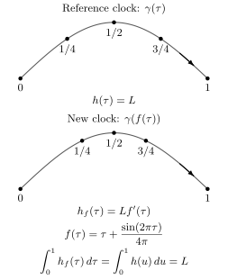
The same kinematical worldline is labeled by two smooth, orientation-preserving clocks. Dots mark ; equal parameter steps need not give equal arclength steps. With reference , the transformed density preserves its integral and the reparametrization-invariant quadratic action. Coordinates and scales agree in both panels. This explicit curve is not asserted to be a free-particle classical solution; is an einbein modulus, not its arclength.
Let us check the invariance explicitly. Under ,
Using , the kinetic term transforms as
where . Similarly,
Therefore .
Constraint and equivalence to the length action
Section titled “Constraint and equivalence to the length action”The einbein is not a propagating field. It has no derivative term. Varying the action with respect to gives an algebraic constraint:
Thus
for and a regular curve with . Substituting this positive solution back into the action gives
Thus the actions agree after classical elimination of in this regular massive domain. This does not by itself define an equality of quantum functional measures; the propagator below will be obtained from a normalized heat kernel. The massless theory still has a useful einbein formulation, but cannot be eliminated by dividing by ; in Lorentzian signature its equation of motion instead imposes the null constraint.
The equation of motion for is
After choosing a gauge in which is constant, this becomes
The classical trajectory is a straight line in flat space, as expected for a free relativistic particle.
The constraint also has a classical Legendre-transform interpretation. The real Euclidean conjugate variable is
At a smooth saddle, the Euclidean einbein equation gives
This real Legendre variable is not the real Fourier variable in the inverse operator . That inverse has no pole on the real Euclidean momentum axis for . After continuation to Lorentzian signature, the physical mass shell in the inherited metric convention is
The Euclidean saddle constraint and the Lorentzian mass shell serve different roles from the spectral denominator used in the heat-kernel construction.
Gauge fixing and the proper-time modulus
Section titled “Gauge fixing and the proper-time modulus”A common trap is to say: since is pure gauge, set
On an infinite line this can be harmless after suitable boundary conditions. But on an interval with endpoints fixed, there is a global invariant:
Under ,
Thus cannot be changed by a reparametrization that preserves the endpoints. The correct local gauge choice is
so that
This fixes the local reparametrization freedom but leaves the modulus . Setting would also fix , which discards an inequivalent value of the modulus. The constant-metric decomposition is described in Polyakov 1987, §9.2, p. 157, Eq. 9.24. His metric component is the square of the einbein used here; the invariant in his notation is the integral of its square root.
With on , the action becomes
Changing variables to proper time gives
This is the form that leads to the Schwinger proper-time representation of a scalar propagator. With the present normalization, the conventional heat-kernel time will be .
Worldline representation of the scalar propagator
Section titled “Worldline representation of the scalar propagator”For a free scalar on with , the Euclidean operator is positive. Its Green function is
To keep the normalization consistent with the gauge-fixed action above, use
for an operator with positive spectrum. Then
The Gaussian Fourier integral fixes the normalization of its massless heat kernel:
It integrates to one in and tends to as . Its path-integral representation is
where the measure is defined by time slicing: each free step of duration uses the factor multiplying its Gaussian. Convolution of these normalized steps gives . Therefore
Equivalently, set and rescale the path parameter. The same expression takes the familiar form
In the variable the free kernel is . As a momentum-space check, the remaining integral is . The position-space Green function is understood as a distribution, or pointwise for ; its coincident limit may require a regulator.
Polyakov’s regulated random-path calculation reaches the Euclidean inverse denominator in Polyakov 1987, §9.2, p. 163, Eq. 9.46. His bare length parameter is tuned to obtain a finite physical mass. The explicit Gaussian integral here fixes our free-field normalization and without equating that bare parameter to .
The two proper-time variables describe the same representation; its structure is
This is the one-dimensional ancestor of the random-surface and string path integrals that appear later. A field propagator can be expanded as a sum over particle paths. A Wilson loop can be treated as a line observable. A confining flux tube suggests a fluctuating surface. The worldline formalism is the cleanest place to see the gauge principle behind all of these statements.
Summary
Section titled “Summary”The first half of the page completed the superconformal-current thread. A chiral supercurrent has weight ,
and its self-OPE closes on the stress tensor,
In modes this gives the super-Virasoro algebra, with the NS relation
The second half shifted from local chiral operators to line geometry. A charged worldline couples to Maxwell theory by the Wilson factor
and the free massive Euclidean particle has the reparametrization-invariant action
The einbein imposes a classical constraint and makes the action quadratic, but endpoint-preserving gauge fixing leaves the positive modulus
Integrating the normalized heat kernel over this modulus, with measure , gives the scalar propagator.
Common pitfalls
Section titled “Common pitfalls”The supercurrent is fermionic. Its modes close under an anticommutator, not an ordinary commutator:
The stress tensor is not an ordinary primary field because of the Schwarzian derivative in finite conformal transformations. The supercurrent is primary under bosonic conformal maps, with weight .
An open Wilson line is not gauge invariant by itself. It becomes gauge invariant only when its endpoints are attached to charged operators, or when the path is closed.
The quadratic worldline action is not the same as the nonrelativistic action unless the einbein gauge and mass-shell constraint are handled correctly. The parameter is gauge, while is a proper-time modulus.
Setting on a finite interval generally overfixes the gauge. The safe gauge is , followed by an integration over in the path integral.
The normalization of the Schwinger parameter must track the normalization of the quadratic action. For , the conventional heat-kernel time is .
The Library treatment of Constraints, Dirac Brackets, and Symplectic Reduction develops the constraint and gauge-reduction machinery behind the worldline action. Its distinction between a constraint surface and the space of physical states clarifies the role of the einbein used here.
Exercises
Section titled “Exercises”The stress tensor acting on the supercurrent
Section titled “The stress tensor acting on the supercurrent”Starting from
using origin-centered counterclockwise mode contours in a fixed NS or R sector, show that
For the inner residue take and a local branch on which the weight is regular. The full weighted outer integrand is single-valued in the chosen sector, so integration by parts has no branch-endpoint term.
Solution
The modes are
The commutator is obtained by moving the contour around :
Using the OPE,
The residues are
and
Therefore
Now insert this into the contour defining :
Integrate the first term by parts:
Thus
Weight of a superdescendant
Section titled “Weight of a superdescendant”In the NS sector, use the supercurrent algebra to show that increases a primary state’s conformal weight by , assuming the descendant is nonzero in the physical quotient.
Solution
Set in
This gives
Let be an eigenstate:
Then
For ,
So creates a superdescendant with conformal weight , unless that descendant is null.
Reparametrization invariance
Section titled “Reparametrization invariance”Verify explicitly that the worldline action
is invariant under the active reparametrization
with , and .
Solution
First compute
Then
Let , so . Then
Similarly,
Both terms in the action are invariant after changing variables from to . Hence
Eliminating the einbein
Section titled “Eliminating the einbein”For , and a smooth Euclidean curve with , eliminate by its equation of motion and show that the classical length action is recovered.
Solution
Varying with respect to gives
For positive and ,
Substitute this back into
The first term becomes
and the second term becomes
Therefore
The surviving proper-time modulus
Section titled “The surviving proper-time modulus”Show that
is invariant under endpoint-preserving reparametrizations.
Solution
Using the active transformation law,
we have
Let . Since and , the integration limits remain and . Thus
So is invariant. This is why gauge fixing can make constant but cannot fix the value of that constant.
Matching the Schwinger parameter
Section titled “Matching the Schwinger parameter”Starting from
set and show that the gauge-fixed path integral has the standard heat-kernel exponent .
Solution
Let , so , , and
The kinetic term becomes
while the mass term becomes
Thus the Euclidean weight is
which is the standard heat-kernel normalization.
Endpoint phases of an open Wilson line
Section titled “Endpoint phases of an open Wilson line”An open Wilson line from to is
Under , find its transformation law and explain how it can be made gauge invariant.
Solution
The exponent changes by
Therefore
For Abelian gauge theory the factors commute, but it is useful to keep the endpoint structure visible. If a charged field transforms as
then the bilocal dressed operator
is gauge invariant, with the phases canceling at the endpoints. A closed Wilson loop has , so the endpoint phases cancel automatically.