

Antiferromagnets, Spin Chains, and Theta Terms
The previous page solved the two-dimensional nonlinear sigma model at large and found a mass gap. That result is the right generic expectation for the model too: the coupling is asymptotically free, grows in the infrared, and usually produces a finite correlation length. But the model has a special extra ingredient in two Euclidean dimensions. Its fields are maps from spacetime into a sphere, and such maps have an integer winding number. The action can therefore contain a theta term.
The Berry phases of microscopic spins determine this term. We derive the leading long-wavelength, large- description of the uniform nearest-neighbor chain, then separate its bulk predictions from the additional hypotheses needed for boundary spins and infrared phases. The resulting action is not merely
but rather
Here is the degree of a smooth map when Euclidean spacetime is closed. For the uniform spin- antiferromagnetic chain,
Thus integer and half-integer spin chains land at different points on the theta circle:
whereas
This is the continuum-field-theory origin of Haldane’s distinction between integer and half-integer antiferromagnetic spin chains.
For readers coming from relativistic QFT, the important conceptual point is that is not chosen by hand in the spin-chain problem. It is fixed by the microscopic spin representation. Changing by changes the interference among topological sectors by a sign.
Required background. Nonlinear sigma models and constraints supplies the kinetic theory, and the large-N saddle explains why the model is generically massive without a topological term. Only the coherent-state Berry phase is new here.
Theta-term normalization and spin-chain dictionary
Section titled “Theta-term normalization and spin-chain dictionary”Spin-chain dictionary
Section titled “Spin-chain dictionary”For the nearest-neighbor antiferromagnetic chain, fix the microscopic spacing , exchange , physical Euclidean time, and unit field . The leading large- dictionary is
| Lattice quantity | Continuum meaning |
|---|---|
| coherent-state spin direction | |
| staggered Néel direction | |
| smooth uniform magnetization density | |
| spin-wave velocity | |
| sigma-model coupling at large | |
| Berry-phase/topological angle |
A consistent rescaling of the auxiliary canting field cancels from the Gaussian integral and does not change these matched and . The approximation requires slow variation on the scale and ; large controls the semiclassical expansion. Small- infrared statements need additional field-theory or microscopic evidence. The original large-spin reduction is developed in Haldane 1983, pp. 1153–1154, Eqs. (5)–(10), PDF.
From a Néel chain to a slowly varying field
Section titled “From a Néel chain to a slowly varying field”Start with an even periodic antiferromagnetic Heisenberg chain, with sites ,
with spin length
Classically, the lowest-energy pattern alternates:
The correct slow variable is therefore not the uniform magnetization, but the staggered Néel field . For a coherent-state unit vector , a length-preserving decomposition is
where
The coherent-state expectation value is . Expanding the square root gives the familiar leading shorthand
The field records the local staggered direction. The smaller field records the smooth ferromagnetic canting, or uniform magnetization density. The two constraints ensure ; the square-root correction matters when deriving coefficients consistently beyond leading order. The figure shows this local orthogonality separately from the alternating microscopic pattern; it does not assume long-range Néel order in the quantum ground state.
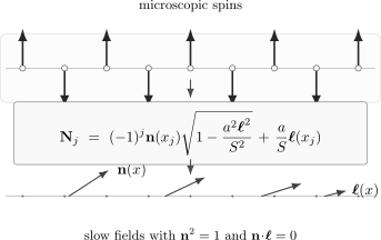
The length-preserving decomposition uses a unit staggered field and a small uniform magnetization density tangent to its sphere. The local arrows share one marked point and satisfy . This is a schematic separation of slow fields, not a ground-state spin configuration or a scale drawing.
To obtain the coefficients, use and . For two neighboring sites, the two square-root corrections and the explicit canting product contribute . A single bond also has an alternating mixed term; averaging the two bonds of an even cell cancels that term at this order. With the slow fields evaluated at the cell center,
Dropping the constant and using gives the continuum Hamiltonian density
The first term says that uniform canting costs energy. The second term says that spatial gradients of the Néel field cost stiffness. The antiferromagnet is special because the time derivative of does not come from the microscopic Hamiltonian alone. It comes from the Berry phase of spin coherent states.
Spin coherent states and the Berry phase
Section titled “Spin coherent states and the Berry phase”A spin- coherent state is labeled by a unit vector and satisfies
The sign follows from the ordered short-time overlap, rather than from a choice between two equivalent-looking phase factors. For spin , take the north-patch state
In , successive resolutions of the identity give
A spin- coherent state is the symmetric product of spinors, so its overlap has times this phase. For a closed trajectory, define the positively oriented solid angle by . The resulting phase is
Because the path-integral weight is , the corresponding term in the Euclidean action is
where is a monopole vector potential on satisfying
This formula is local only in patches on the sphere. The solid angle is defined modulo , so the phase is well-defined precisely because is an integer:
The overlap construction agrees with Altland and Simons 2023, § 8.4.5, pp. 449–451, Eqs. (8.21)–(8.26): their Euler-gauge state becomes this north-patch state after multiplication by . This adds to their connection . The figure fixes the orientation by a positive latitude traversal.
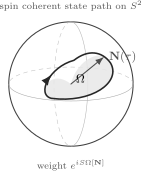
The positively traversed latitude at bounds the displayed north-pole cap, with . Ordered Euclidean overlaps contribute , equivalently the action ; the spin-half phase in this example is . This north-pole projection is schematic; the solid-angle formula is exact. The ambiguity is harmless because .
For a whole spin chain, the coherent-state path integral contains
where is the direction of the spin at site . In an antiferromagnet,
For positive target curvature the variation is . Inserting around either or gives the same contribution, . Multiplication by and summation over sites therefore give
Combining this with the continuum Hamiltonian density gives, to leading order,
The field is Gaussian. Integrating it out gives
At fixed , integrate over the two real tangent components of . For this is a convergent Gaussian. Completing the square gives the imaginary stationary point and the positive time-derivative term above; the contour translation is justified by the entire Gaussian integrand and its decay. The field-independent determinant cancels in normalized observables.
This can be written in relativistic-looking form
with
These are the leading large- coefficients for the stated microscopic normalization; see Fradkin 2013, § 7.5, pp. 202–204, Eqs. (7.57)–(7.71). After setting , this becomes the ordinary two-dimensional nonlinear sigma model,
The remaining, alternating part of the Berry phase is the topological term. It is here that the microscopic spin length survives in a way no local gradient expansion could guess.
Ferromagnets and antiferromagnets use Berry phases differently
Section titled “Ferromagnets and antiferromagnets use Berry phases differently”For a ferromagnet, neighboring spins point in nearly the same direction, so their Berry phases add. The continuum Euclidean action begins schematically as
The time derivative is first order. After continuation to real time, it pairs the two transverse spin-wave coordinates as conjugate variables and gives the quadratic magnon dispersion .
For an antiferromagnet, the leading Berry phases alternate and nearly cancel. Their smooth remainder couples to ; integrating out the costly canting field produces . The semiclassical dispersion is therefore linear, . The cancellation is not complete: its quantized remainder is the theta term derived next.
How the theta term appears
Section titled “How the theta term appears”The Berry phase is sensitive to the fact that neighboring antiferromagnetic spins live near opposite points on the sphere. Pair neighboring sites. The Berry phases of the two spins nearly cancel, but their small mismatch is a total derivative in field space. Summed over the chain, these mismatches become the winding number of the map .
Varying the north-patch one-form and integrating its term by parts gives
Taking gives
Using cyclic symmetry of the scalar triple product,
Use modulo . An even site and its following odd neighbor contribute , the negative of the difference above. There is one such pair per length , so
The arrow denotes the leading gradient limit; higher-gradient corrections have been dropped. Thus the Euclidean action contains , with
For the uniform chain, the coefficient is fixed by the quantized microscopic spin representation. Choosing the other sublattice for reverses and the corresponding theta convention; keep the termination as well when comparing open chains. The continuum phase remembers whether the microscopic spin is integer or half-integer, even though the kinetic coefficients alone do not encode that parity.
Topological charge as degree
Section titled “Topological charge as degree”Before using the theta term, it is worth seeing why is an integer. Start with the simpler case. A path on a circle may be written as
with periodicity of the physical point
The angle itself may wind:
The winding number is
The topological charge is the two-dimensional version of this statement. On the Euclidean plane, impose at infinity and sufficient regularity for the field to extend smoothly to the one-point compactification,
Finite action alone does not imply this boundary condition. For example, a field that equals for , smoothly completed inside, has a finite energy tail proportional to , yet has no limit at infinity. With the stated compactification hypothesis, a field configuration is a map
Such maps have an integer degree. In angular coordinates on the target sphere,
one finds
Therefore
This is the signed target-sphere area swept out by the map, divided by the area of the unit sphere. For a regular target point, count its preimages with the signs of their local Jacobians. The signed count is the degree; pulling back the sphere’s area form and summing those oriented sheets gives times that integer. A configuration that covers the target sphere once with positive orientation has . The figure shows the domain hypothesis that licenses this interpretation.
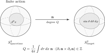
With a fixed limiting field and a smooth extension at infinity, the plane becomes a compact domain . The degree of is the signed target area divided by . Finite action by itself is insufficient. The spheres and arrow are schematic; the orientation and normalization of are explicit.
On a closed spacetime, the theta term does not change the local classical equations of motion for smooth variations within a fixed topological sector. It multiplies sectors by phases:
where is the contribution from configurations of topological charge . Since is integer on a closed oriented spacetime,
Boundaries and edge Berry phases
Section titled “Boundaries and edge Berry phases”The statements “ is an integer,” “ is -periodic,” and “the theta term does not affect the local variation” all require a qualification when spacetime has a boundary. Orient the thermal strip , with periodically identified, by , as in the bulk convention above, and use the outward-normal-first rule on . The left boundary is then traversed with increasing , while the right boundary is traversed with decreasing . Let and denote the solid angles swept by the two endpoint fields when each is parametrized with increasing , using the same target-sphere orientation as the single-spin Berry phase above. After attaching orientation-compatible caps, Stokes’ theorem gives
The integer changes when a different cap is chosen, while the full microscopic Berry factor remains unambiguous. Substituting shows that the boundary-dependent part of the Euclidean action is
For an integer-spin chain with a gapped Haldane bulk and the corresponding open termination, these are the Berry actions of two effective spins with opposite boundary orientations. The right-hand minus sign can be represented by an edge direction . The closed-bulk factor is then trivial, while the edge factors need not be. The open spin-1 valence-bond construction exhibits the spin- endpoints explicitly; see Affleck, Kennedy, Lieb and Tasaki 1987, pp. 799–801, PDF.
The integer-spin hypothesis matters. Changing the left cap sends and , leaving the full unchanged. The isolated edge factor would instead acquire . It is single-valued for integer but changes sign for half-integer . A gapless spin-half bulk therefore does not supply an autonomous spin-quarter edge: the bulk and boundary expression must be retained together.
The protected information is the projective symmetry class of the edge, rather than a fixed multiplet for every boundary Hamiltonian. For odd integer , the half-integer edge is projective under and has Kramers degeneracy under physical time reversal. For even integer , an integer-spin boundary multiplet can be screened or replaced by a singlet without closing the bulk gap. These statements assume the protecting symmetry and a gapped bulk; Pollmann, Berg, Turner and Oshikawa 2012, arXiv v3, § III.A, pp. 3–4, PDF explains the edge-level distinction.
This resolves an apparent contradiction. The bulk values and give the same partition function on a closed spacetime, yet they can encode different boundary physics when the protecting symmetries are retained. Theta periodicity should therefore never be used to erase an open chain’s boundary Berry phases.
Integer and half-integer spin
Section titled “Integer and half-integer spin”Combining
with closed-spacetime theta periodicity gives two possible topological phases in the microscopic weight:
At , the closed-bulk model behaves like the ordinary asymptotically free sigma model. The coupling grows in the infrared and the theory produces a mass gap,
up to prefactors and scheme-dependent definitions of the ultraviolet scale. For the uniform nearest-neighbor chain and its Haldane phase, this gives the leading semiclassical explanation of the integer-spin bulk gap. It is not a proof of the microscopic gap for every from the gradient expansion. The bulk statement also does not remove the boundary degrees of freedom of an open chain.
At , the topological sectors enter with the sign
Even and odd sectors enter with opposite signs; this does not imply that their magnitudes cancel exactly. For the uniform nearest-neighbor spin- Heisenberg antiferromagnet, the infrared fixed point is the Wess–Zumino–Witten conformal field theory, with logarithmic corrections from a marginally irrelevant operator. In a one-dimensional spin system with finite-range interactions at zero temperature in the thermodynamic limit, the Lieb–Schultz–Mattis constraint rules out a unique symmetry-preserving gapped ground state with half-odd-integer spin per unit cell and unbroken one-site translation and spin-rotation symmetry. A gapless phase and symmetry-breaking ground-state degeneracy are distinct alternatives; the theta angle alone does not select between all possible microscopic Hamiltonians. See Affleck and Haldane 1987, pp. 5294 and 5297, PDF.
The figure separates this uniform-chain classification from the effect of explicit bond alternation discussed next. Its arrows express the stated implications, not trajectories in a computed coupling plane.
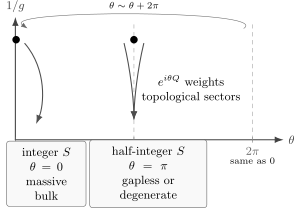
For the uniform chain, the microscopic spin fixes ; periodicity reduces it to or on closed spacetime. The ordinary sigma model is massive, and the nearest-neighbor spin-half chain at is critical. More general half-integer chains obey the symmetry obstruction stated in the text. Explicit dimerization breaks one-site translation while preserving physical time reversal and can open a gap. This is a schematic classification, not an RG-flow calculation; open-chain edges require the separate boundary action.
This is a striking lesson. The local Lagrangian density
has the same local form for and , although its matched coupling differs. It does not encode the quantized integer/half-integer interference. That information lies in a topological phase invisible in ordinary perturbation theory around a smooth trivial-sector configuration.
Symmetry constraints on the theta angle
Section titled “Symmetry constraints on the theta angle”The antiferromagnetic chain has microscopic symmetries that act nontrivially on the continuum field. A one-site translation reverses the Néel field:
The topological density changes sign under this map because
so
Because translation is unitary, the path-integral phase can be invariant under this transformation only when
which requires
These two symmetry-invariant values are precisely the two values realized by uniform integer and half-integer antiferromagnetic spin chains.
Physical time reversal reverses spins and the temporal ordering of a history. For an antiunitary operator ,
For a periodic sequence of states , set . Each transformed overlap is , so the cyclic product is unchanged. Complex conjugating this reversed product once more would count the reversal twice. The corresponding field history is ; its topological density is . Physical spin time reversal therefore does not impose the same restriction on as unitary one-site translation.
A concrete check is the spin-half alternating chain
Every exchange product is time-reversal invariant, for any real . One-site translation instead sends . With even bonds chosen strong for , the alternating mixed bond term no longer cancels. At the same gradient order the Hamiltonian density is
Shift the real tangent field by . Its Berry coupling then leaves the extra action . Combining it with gives at this matching order. For spin half,
This follows from Foussats, Greco and Muramatsu 2011, § 4, pp. 235–239, Eqs. (4.1), (4.22)–(4.24), PDF. Their topological integral is in our normalization, so its coefficient gives the expression above. For example, preserves physical time reversal while giving . Bond alternation is relevant near the uniform spin-half critical chain and opens a gap; the doubled cell contains integer total spin, so the one-site Lieb–Schultz–Mattis obstruction no longer applies. This continuum matching does not by itself determine the gap at arbitrary strong dimerization.
A local coordinate check
Section titled “A local coordinate check”Locally, the field has only two independent components. Choose a patch near the north pole and write
Then
So the two local fields are the spin-wave coordinates. At weak coupling, after rescaling , the leading interaction is order . This is the same perturbative sigma-model expansion used on the previous pages.
The topological term is different. In a single coordinate patch, it looks like a total derivative or a curl. On a closed spacetime it does not change the perturbative beta function of at any finite order. With a boundary, the same total derivative is precisely why a boundary term remains. Globally, no single smooth coordinate patch covers all configurations of nonzero . The theta term can therefore be invisible in bulk perturbation theory and still decide the infrared and edge physics.
Relation to the next step
Section titled “Relation to the next step”The continuum antiferromagnet raises a question that sounds paradoxical at first. The microscopic classical picture has a Néel vector, but the one-dimensional quantum chain has no ordinary long-range staggered magnetization in its symmetric ground state. In field-theory language, low-dimensional fluctuations restore the continuous symmetry.
The next page studies this symmetry restoration more directly. It returns to the sigma model as a quantum field theory and explains why the order parameter vanishes even when the classical field wants to choose a point on the sphere.
Summary
Section titled “Summary”A one-dimensional antiferromagnetic Heisenberg spin chain has low-energy variables
The exchange interaction gives spatial stiffness and a cost for uniform canting. The spin coherent-state Berry phase gives the time derivative term and, more importantly, the theta term. After integrating out , the low-energy Euclidean action is
with
The topological charge is
Thus integer spin gives modulo and the ordinary massive bulk sigma-model behavior, while half-integer spin gives modulo . The nearest-neighbor spin- chain is critical; more generally, the half-odd-integer chain cannot be a trivial unique symmetric gapped state. On an open chain, the bulk periodicity must be supplemented by the endpoint Berry phases, which retain information that a closed-spacetime reduction would discard.
Common pitfalls
Section titled “Common pitfalls”Forgetting the Berry phase. The ordinary gradient energy only produces the sigma-model kinetic term. The integer versus half-integer distinction comes from the spin coherent-state Berry phase.
Mixing the Berry factor with the Euclidean action. With the positive-curvature solid angle used here, ordered coherent-state overlaps give and the Euclidean action is . Derive the variation and the canting coupling using that same orientation.
Treating the theta term as a small local perturbation. It weights entire topological sectors by phases . Its leading density can be a total derivative in one patch while its global effect remains nonperturbative.
Losing the factor of . The spin-chain result is , not . Since is periodic modulo on closed spacetime, this factor is exactly what separates integer from half-integer bulk theories.
Using closed-spacetime periodicity on an open chain. When there is a boundary, need not be an integer by itself and the theta term leaves endpoint Berry phases. In particular, reducing to zero before retaining the boundary term erases the spin- edges of the spin-1 Haldane chain.
Overstating the gapless claim. The uniform nearest-neighbor spin- Heisenberg antiferromagnet is critical, but the general half-odd-integer constraint allows either gaplessness or degeneracy. Explicit dimerization can open a gap because it doubles the unit cell and breaks one-site translation.
The Library treatment of Antiferromagnets, Sigma Models, and Theta Terms develops the spin-chain application of the Berry-phase and theta-term construction. Compare the stated Berry-curvature orientation and boundary conditions before identifying the two actions.
Exercises
Section titled “Exercises”Exercise 1: integrating out the uniform magnetization
Section titled “Exercise 1: integrating out the uniform magnetization”Starting from
with , , and , complete the tangent-plane Gaussian square and show that the time-derivative term is
Solution
The -dependent part is
The stationary point satisfies
so
Completing the square,
Since , we have
and therefore
Thus integrating out gives
Exercise 2: topological charge of the identity map
Section titled “Exercise 2: topological charge of the identity map”Let the domain sphere have coordinates with and . Consider the identity map to the target sphere,
Show that .
Solution
For this parameterization,
Therefore
The integrals give
Thus
The identity map covers the target sphere exactly once with positive orientation.
Exercise 3: the boundary term at θ = 2πS
Section titled “Exercise 3: the boundary term at θ = 2πS”For an integer-spin chain in a gapped Haldane regime with the open termination described above, suppose the capped topological charge is
Insert into . Identify the two edge Berry actions and the spin-1 example. Why would separating off an autonomous spin- edge fail for microscopic ?
Solution
Substitution gives
The second term is
The signs reflect the opposite boundary orientations. For , the bulk factor , while the two endpoints have spin- Berry actions. This identifies their projective edge class in the stated gapped regime. For microscopic , changing one cap by multiplies its isolated spin-quarter phase by . The compensating change restores the full strip phase, so the separate edge factor is not an autonomous spin path integral.
Exercise 4: translation and the topological charge
Section titled “Exercise 4: translation and the topological charge”A one-site translation acts on the Néel field as . Show that this sends . For which theta angles is the phase invariant under this transformation for all ?
Solution
Under ,
The cross product of two derivatives is unchanged:
But the remaining factor of changes sign, so
Therefore
The phase is invariant if
for all integers . This requires
for all , hence
Modulo , the solutions are
Exercise 5: why the theta term is invisible in small-field perturbation theory
Section titled “Exercise 5: why the theta term is invisible in small-field perturbation theory”In a local patch write
Count derivatives at the same small-field amplitude order as the fields. Show that the topological density begins with a total derivative:
Then rewrite the leading term as a total derivative and explain what changes when spacetime has a boundary.
Solution
To leading order,
so
and
The leading cross product points in the first internal direction:
Dotting with gives
The leading term is
because mixed derivatives commute. On a closed spacetime, or for fluctuations that vanish at infinity, the integral of this term vanishes. With a boundary it instead leaves a boundary contribution, consistent with the endpoint Berry phases derived above. This is why the theta term does not modify ordinary bulk perturbation theory around the trivial sector while remaining physically important.
References
Section titled “References”- I. Affleck and F. D. M. Haldane, “Critical Theory of Quantum Spin Chains,” Physical Review B 36 (1987) 5291–5300, doi:10.1103/PhysRevB.36.5291. Open PDF.
- I. Affleck, T. Kennedy, E. H. Lieb, and H. Tasaki, “Rigorous Results on Valence-Bond Ground States in Antiferromagnets,” Physical Review Letters 59 (1987) 799–802, doi:10.1103/PhysRevLett.59.799.
- A. Altland and B. Simons, Condensed Matter Field Theory, 3rd ed., Cambridge University Press, Cambridge, 2023, doi:10.1017/9781108781244.
- A. Foussats, A. Greco and A. Muramatsu, “Path Integrals for Dimerized Quantum Spin Systems,” Nuclear Physics B 842 (2011) 225–247, doi:10.1016/j.nuclphysb.2010.09.001. Open PDF.
- E. Fradkin, Field Theories of Condensed Matter Physics, 2nd ed., Cambridge University Press, Cambridge, 2013, publisher record.
- F. D. M. Haldane, “Nonlinear Field Theory of Large-Spin Heisenberg Antiferromagnets: Semiclassically Quantized Solitons of the One-Dimensional Easy-Axis Néel State,” Physical Review Letters 50 (1983) 1153–1156, doi:10.1103/PhysRevLett.50.1153.
- F. Pollmann, E. Berg, A. M. Turner and M. Oshikawa, “Symmetry Protection of Topological Phases in One-Dimensional Quantum Spin Systems,” Physical Review B 85 (2012) 075125, doi:10.1103/PhysRevB.85.075125. Open PDF, arXiv:0909.4059v3.
Further reading
Section titled “Further reading”- F. D. M. Haldane, “Continuum Dynamics of the 1-D Heisenberg Antiferromagnet: Identification with the O(3) Nonlinear Sigma Model,” Physics Letters A 93 (1983) 464–468, doi:10.1016/0375-9601(83)90631-X.
- E. H. Lieb, T. Schultz, and D. Mattis, “Two Soluble Models of an Antiferromagnetic Chain,” Annals of Physics 16 (1961) 407–466, doi:10.1016/0003-4916(61)90115-4.
- A. M. Polyakov, Gauge Fields and Strings, Contemporary Concepts in Physics, Vol. 3, Harwood Academic Publishers, Chur, 1987.
- A. Zee, Quantum Field Theory in a Nutshell, 2nd ed., Princeton University Press, Princeton, 2010.