

Lattice Dirac Equations and Euclidean Spinors
The Ising order–disorder field obeys an exact lattice difference equation whose critical, long-wavelength limit is a Euclidean Dirac equation. Three steps make this statement useful in calculations: scaling the source together with the lattice operator, distinguishing a Lorentzian mass-shell spinor from a Euclidean field, and carrying the spinor basis through Wick rotation. This lesson works through those steps and then explains why three-dimensional Ising duality introduces gauge variables.
The calculation uses the transported disorder cuts of lesson 8 and the explicit four-corner projection, mass normalization, and Euclidean gamma matrices of lesson 9.
From disorder endpoints to corner spinors
Section titled “From disorder endpoints to corner spinors”In the zero-field Ising model, a disorder insertion changes the signs of the couplings on bonds crossed by a dual-lattice path. Paths connect disorder endpoints in pairs or terminate at a specified boundary. For a chosen collection of paths ,
A contractible deformation of can be implemented by flipping spins in the enclosed region. The disorder correlator is unchanged unless that deformation crosses an order insertion, which contributes a minus sign. On a periodic lattice, winding classes and boundary sectors must also be specified; path independence is not permission to change them. These qualifications follow directly from the bond-sign definition and spin change of variables Kadanoff and Ceva 1971, pp. 3919–3921.
Let be an original-lattice site and one of its four neighboring dual sites. With lattice spacing , use the lifted corner angles
The corner field is the point-split composite
Transporting its disorder cut once around the order insertion produces the continuation rule
The angle is lifted along the transport: replacing it by a principal value after a full turn would erase precisely this sign. Four independent corner values have four antiperiodic characters,
The labels are character classes modulo , not an infinite set of independent lattice fields. The critical pair is . Its continuum normalization is the common factor found in lesson 9:
Thus the raw Fourier coefficients should not also be called the normalized continuum fields. The other two combinations have a nonzero lattice gap at criticality; eliminating them produces higher-derivative corrections. The local relation, antiperiodicity, and critical projection are developed in Polyakov 1987, § 10.3.1, pp. 276–278.
In the figure, distinguish the short corner displacement from the extended disorder cut. The cut must be transported along with its endpoint; the short arrow alone does not specify that cut.
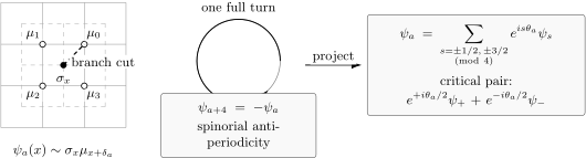
The solid short arrow is the corner displacement; the dashed dual-lattice path is a reference disorder cut continued outside this schematic patch. Hollow markers show alternative corner endpoints. Transporting the cut through gives . The four raw Fourier coefficients use the same lifted angles as lesson 9, which supplies the normalization of the critical pair.
The preceding lesson already projected the exact Ising relation. A scalar example now isolates a separate issue that matters equally for spinors: which quantities must scale when a lattice equation becomes a continuum equation.
Lattice Green functions and source normalization
Section titled “Lattice Green functions and source normalization”Consider a scalar field on an infinite one-dimensional lattice, indexed by . This is an illustrative scalar operator, not the full Ising fermion kernel. Its dimensionless equation is
The positive mass makes the inverse well-defined; the massless case requires separate control of the zero mode and infrared behavior. Fourier-transform with dimensionless momentum :
Shifts of multiply the Fourier field by , so
Near , the symbol has the expansion
To take a physical continuum limit, set
Here samples without an additional field rescaling. Dividing the whole equation, including its source, by gives
For smooth fields at fixed physical ,
The source scaling is essential: keeping fixed while dividing the left side by would produce a divergent physical source. The corresponding physical Green operator has symbol .
Inspect the difference between the exact symbol and its quadratic approximation in the figure. Agreement is local in momentum, not uniform across the Brillouin zone.
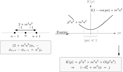
The stencil requires , , , and . The quantitative plot compares the exact symbol with its quadratic approximation at fixed . It is a one-dimensional symbol, also the slice of the square-lattice scalar symbol. Dividing the equation by gives the physical continuum operator for and .
A controlled low-energy approximation requires sources and observables restricted to small lattice momenta, , and . These are spectral conditions; a pointwise condition such as is not a useful general test, since even a smooth field may cross zero. For this example the exact decay length obeys
The first identity follows from the nearest pole at , where . It makes the scale separation explicit. The analogous Ising Dirac limit keeps a physical mass fixed while tuning proportionally to ; an exact lattice identity alone does not justify that limit far from criticality.
The Dirac equation in light-cone variables
Section titled “The Dirac equation in light-cone variables”In two Lorentzian dimensions, write the physical contravariant momentum as and define
Use the chiral gamma matrices
The covariant momentum is , so the momentum-space Dirac equation is
For this means
The determinant condition is
It is necessary for a nonzero solution; the first-order equation also fixes the relative components. On the positive-energy massive shell, with real , both are positive and a solution is
Indeed, , so the relative sign is required when . The normalization is independent of this algebraic check. This formula is not a prescription for the negative-energy shell. At , the equations instead separate into chiral branches: for , , whereas for , .
A boost with
acts as . Its spin representation is
One can verify directly that . On the positive-energy shell the square roots above give the same transformation with a fixed common phase. Thus the half-rapidity factors follow from covariance of the equation, including when a square-root parametrization is unsuitable.
Wick rotation with a fixed spinor basis
Section titled “Wick rotation with a fixed spinor basis”Wick rotation changes both the momentum dictionary and the convenient spinor basis. To match the Euclidean gamma matrices and active rotations of lesson 9, use
This matches the Fourier phases on the complexified variables. It states the local algebraic continuation; a correlation-function Wick rotation additionally requires the appropriate analyticity, boundary conditions, and pole prescription.
Define Euclidean complex momenta by
The Lorentzian light-cone components then become
They do not become a conjugate pair with the same signs. After this substitution, change basis with
Direct multiplication gives
Thus and, in position space,
For an active counterclockwise Euclidean rotation , the continuation of the stated boost is . Therefore
This is exactly the active convention used in lesson 9. It is compatible with , and recovers the transported corner sign. The figure follows this particular continuation through each change of variables.
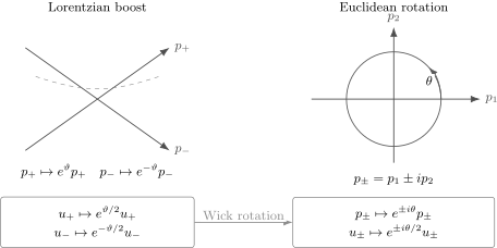
Lorentzian light-cone momenta transform as . With , , and , their continuation gives . The continuation yields the active Euclidean spinor phases . These are transformation laws; they do not assert a real Euclidean massive mass shell.
That last distinction is consequential. For real Euclidean and real nonzero ,
There is no nonzero homogeneous on-shell spinor at such a momentum. Euclidean fields and Green functions are perfectly well-defined, but assigning their components the real-momentum expressions would not solve the massive equation. The half-angle law follows from the spin representation, independently of such roots.
The Euclidean Majorana action is a quadratic form in independent Grassmann fields with antisymmetric kernel , where and transposition includes integration by parts. Its integral is a Pfaffian once the Grassmann integration order is fixed. In this complex chiral basis the kernel need not be entrywise real; one should not impose a pointwise relation . Lesson 9 gives the compatible local action and explains its global-sector limitations.
With the same Ising projection and lattice spacing,
Here is the free-fermion decay length in the chosen continuum normalization. Other correlation channels may have different amplitudes. Kramers–Wannier duality reverses this signed mass to leading order; the mass gap remains nonnegative.
Why three dimensions lead to gauge variables
Section titled “Why three dimensions lead to gauge variables”For a finite Ising graph with all site spins summed and no magnetic field, expand every bond factor as
Each term chooses a bond subset . Summing a spin gives zero unless an even number of chosen bonds meet that vertex. Hence, in any dimension,
Here means even incidence modulo , counts sites, and counts bonds. The graphs can have intersections and even-valence junctions; they need not be disjoint simple loops.
The low-temperature expansion uses different objects. On a connected periodic cubic lattice, assign dual cubes to the minus spins and call their union . The frustrated bonds correspond to the dual plaquette boundary . Since , every dual link has even plaquette incidence. The surface is a boundary of a spin region, not necessarily a smooth embedded manifold. Each such boundary corresponds to two globally reversed spin configurations, giving
The notation means precisely the plaquette sets that bound a union of dual cubes. Thus three-dimensional low-temperature spin configurations produce two-dimensional surfaces, whereas high-temperature site-spin graphs remain one-dimensional. The appropriate dual local variables are gauge fields on links Wegner 2014, § 3, p. 5 (PDF).
Put on each link of the dual cubic lattice and define
This sum includes every link assignment, without dividing by the gauge-group volume. Expand the plaquette factors and sum links. A plaquette subset survives precisely when every link occurs an even number of times:
Here count the gauge links and plaquettes; denotes all closed plaquette sets modulo . Four occupied plaquettes can meet along a link, so “closed surface” does not require a manifold neighborhood there.
The figure distinguishes this local closure condition from the global condition of bounding a spin region.
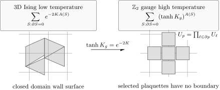
Spin domain walls are boundaries . Gauge high-temperature selections are plaquette cycles modulo , requiring even incidence at every link. The middle cross-section shows two closed cube boundaries sharing an edge with four incident plaquettes; the lower periodic plane is closed but does not bound a periodic spin domain. These schematic examples distinguish local weight matching from exact duality with compatible boundaries and sectors.
Matching the weight of a selected plaquette gives
This local relation is necessary, but on a three-torus it is not by itself an equality of the two partition functions just written. A single plane wrapping the torus belongs to and does not belong to . Exact finite-volume duality must match the allowed boundary conditions or sum over the required twisted sectors, as well as include the prefactors. On a contractible cubical complex all closed two-cycles bound, but the boundary spin and gauge sums must still be chosen consistently. The closure and completeness conditions, normalization, and explicit periodic-boundary example are treated in Wegner 2014, § 4, pp. 7–9, Eqs. (20)–(39) (PDF).
The geometric mechanism is now precise: link sums select plaquette cycles with the same local weight as spin domain walls. The next lesson develops the gauge symmetry and Wilson loops of this system.
Common pitfalls
Section titled “Common pitfalls”Forgetting the source scaling. Dividing a lattice operator by also divides its source. State the normalization of both before taking the limit.
Reusing light-cone labels after Wick rotation. The dictionary here is and , followed by a fixed basis change. Dropping that minus sign changes the Euclidean operator.
Using mass-shell roots for Euclidean fields. The positive-energy Lorentzian root formula has a declared mass sign and branch. Euclidean rotation weights remain meaningful even when no nonzero massive homogeneous solution exists at real momentum.
Equating closed surfaces with spin boundaries. Local even incidence is a closure condition. Periodic lattices also support closed surfaces that wrap a nontrivial cycle and cannot arise as the boundary of a periodic spin domain.
The Library treatment of The Dirac Field provides the continuum action, current and spinor identities that complement this lattice construction. Apply the lesson’s stated Euclidean continuation and field dictionary before comparing its lattice components with Lorentzian spinors.
Exercises
Section titled “Exercises”Exercise 1: The lattice Green function
Section titled “Exercise 1: The lattice Green function”Fourier-transform
Derive the exact Fourier Green function, its physical continuum limit, and the required source scaling. Check the leading correction to the symbol.
Solution
The two shifts contribute and . Therefore
With and ,
The inverse physical operator is thus at fixed . Since the field is sampled without further rescaling, dividing the position-space equation by requires . The result is . Holding the lattice source fixed would not implement this limit.
Exercise 2: Light-cone Dirac kinematics
Section titled “Exercise 2: Light-cone Dirac kinematics”Show that a nonzero solution of requires . Check the positive-energy root formula for both signs of , and verify boost covariance directly.
Solution
The determinant is . It must vanish for a nonzero kernel, including when one spinor component vanishes. On the positive-energy massive shell, and . Consequently
These are the two equations for . Omitting the relative sign fails for negative mass.
Under , the off-diagonal entries of are and , identical to those of . Their diagonal entries also agree. Thus a solution transforms by . This covariance statement also applies to the massless chiral branches, for which the massive square-root parametrization need not be used.
Exercise 3: Continuation and the Euclidean spinor sign
Section titled “Exercise 3: Continuation and the Euclidean spinor sign”Use , , and to derive . Continue the boost by and check the full-turn sign. Explain why this does not give massive on-shell spinors at real Euclidean momentum.
Solution
The continued light-cone variables are and . Multiplying by and gives
Since and are diagonal,
The derivative operator is covariant: . The full-turn sign characterizes the representation. It does not require to have a kernel at real : indeed for real nonzero .
Exercise 4: Why three-dimensional spin duality changes form
Section titled “Exercise 4: Why three-dimensional spin duality changes form”Explain why the high-temperature spin expansion uses even bond subgraphs in any dimension. For a periodic three-dimensional lattice, characterize the low-temperature objects and explain why they require different dual local variables.
Solution
Expanding each selects occupied bonds. At a vertex of degree in that selection,
Thus the surviving selections are one-dimensional even subgraphs in every dimension. Even-valence junctions are allowed.
In three dimensions, let be the dual cubes corresponding to minus spins. Unsatisfied bonds correspond to plaquettes in , with weight . These objects are two-dimensional boundaries modulo ; four plaquettes may meet along a link. Periodicity further excludes a lone nonbounding wrapping plane from a periodic spin configuration.
A site-spin high-temperature expansion produces bond graphs, not these plaquette objects. Link variables with plaquette interactions give the appropriate local dual description, subject to matching the global sectors.
Exercise 5: Gauge-theory surfaces and normalization
Section titled “Exercise 5: Gauge-theory surfaces and normalization”For , derive the complete high-temperature prefactor and cycle sum. Explain the additional condition needed to compare it with periodic Ising domain walls.
Solution
Expand each plaquette factor as , where . A selected plaquette subset contributes
Each link sum is zero for odd and for even . Therefore
The closure condition is modulo and permits intersecting plaquette cycles. The factor is correct because the original partition function sums all link configurations.
Matching local plaquette weights gives . Periodic Ising walls, however, lie in , whereas the gauge expansion sums . A nonbounding wrapping plane belongs only to the latter. One must match the boundary or twisted-sector sums, and retain the different prefactors, before asserting an exact finite-volume partition-function identity.
References
Section titled “References”- Kadanoff, L. P., and H. Ceva. “Determination of an Operator Algebra for the Two-Dimensional Ising Model.” Physical Review B 3, 3918–3939 (1971). DOI: 10.1103/PhysRevB.3.3918.
- Polyakov, A. M. Gauge Fields and Strings. Harwood Academic Publishers, 1987. § 10.3.1, pp. 276–278. DOI: 10.1201/9780203755082.
- Wegner, F. J. “Duality in Generalized Ising Models.” arXiv:1411.5815v1 (2014). §§ 3–4, pp. 5, 7–9. Stable record; Open PDF.
Further reading
Section titled “Further reading”- Kogut, J. B. “An Introduction to Lattice Gauge Theory and Spin Systems.” Reviews of Modern Physics 51, 659–713 (1979). DOI: 10.1103/RevModPhys.51.659.
- Wegner, F. J. “Duality in Generalized Ising Models and Phase Transitions without Local Order Parameters.” Journal of Mathematical Physics 12, 2259–2272 (1971). DOI: 10.1063/1.1665530.