Renormalization and Running Couplings

A loop diagram is an instruction to sum over virtual fluctuations at all momenta allowed by the theory. The high-momentum part of that sum probes distances much shorter than the wavelength of the external particles. From far away, a tiny loop cannot be resolved: it looks like a point. This is the basic reason ultraviolet divergences are not arbitrary monsters. They are local.

The previous page used one-loop diagrams and power counting to identify which ultraviolet divergences can occur. This page turns that observation into the renormalization group. A local divergence can be absorbed into the coefficient of a local operator. Once the coefficient has been fixed at one scale, the same physical amplitude at another scale contains logarithms. Those logarithms are most cleanly described by allowing masses, fields, and couplings to depend on the scale at which they are defined.

Renormalization is therefore not merely a trick for subtracting infinity. It is the statement that a quantum field theory is specified by a choice of local operators and a rule for how their coefficients change when the resolution scale changes.

Two scale variables will appear. A Wilsonian cutoff $\Lambda$ describes which modes are still present in an effective action. A renormalization scale $\mu$ describes where finite parameters are defined after a subtraction prescription has been chosen. They are related, but not identical. Confusing them is one of the fastest ways to get the sign of an RG flow wrong.

Ultraviolet subgraphs are local

This lesson preserves the lecture sequence and develops renormalization from local ultraviolet subgraphs. Ultraviolet Sensitivity and the Renormalization Problem develops the canonical locality and input-setting treatment; Renormalization- Group Equations and Running separates subtraction-scale evolution from Wilsonian coarse graining.

Wilsonian cutoff versus subtraction scale

This page uses a Euclidean UV cutoff $\Lambda$ to explain locality and running. A Lorentzian Feynman integral is first defined by its $+i0$ prescription; when its contour can be deformed without crossing a singularity, it is Wick-rotated and the compact cutoff is then imposed as $k_E^2\leq\Lambda^2$. A compact hard cutoff is not Lorentz invariant in Minkowski momentum space. The same physics can be expressed in dimensional regularization and minimal subtraction, where logarithms of $\Lambda$ are replaced by poles in $4-d$ and logarithms of the subtraction scale $\mu$. Allowed operator structures agree once the symmetries are enforced. Couplings and beta functions depend on their definitions and transform together under a change of renormalization scheme; physical predictions must agree after matching those definitions.

Before imposing the cutoff, a one-loop subgraph with external momenta $p_i$ and loop momentum $k$ has the typical Lorentzian structure

$$I_L(p_i)=\int {d^4k\over(2\pi)^4}\, {N(k,p_i)\over \prod_a\left((k+P_a(p_i))^2-m_a^2+i0\right)}.$$

The $+i0$ fixes the contour deformation. After an allowed Wick rotation, the regulated integral is schematically

$$I_E(p_{i,E})= \int_{k_E^2\leq\Lambda^2}{d^4k_E\over(2\pi)^4}\, {N_E(k_E,p_{i,E}) \over \prod_a\left((k_E+P_{a,E})^2+m_a^2\right)}.$$

The ultraviolet region is $|k_E|\gg |p_{i,E}|,m_a$. In that region the Euclidean integrand can be expanded in powers of the small ratios $p_{i,E}/k_E$ and $m_a/k_E$:

$${N_E(k_E,p_{i,E}) \over \prod_a\left((k_E+P_{a,E})^2+m_a^2\right)} =\sum_{r=0}^{R} {\mathcal P_r(p_{i,E},m_a;\widehat k_E)\over |k_E|^{\alpha_r}} +\text{terms convergent as } |k_E|\to\infty .$$

After $O(4)$ angular integration, the divergent terms are polynomials in the external momenta and masses. A polynomial in momentum space is a finite number of derivatives in position space, so the divergent part has the form of a local operator:

$$I_{\mathrm{div}}(p_i) =c_0(\Lambda)+c_2(\Lambda)p^2+c_4(\Lambda)p^4+\cdots .$$

The coefficients $c_r(\Lambda)$ may diverge as powers of $\Lambda$ or as $\log \Lambda$, but the dependence on the slowly varying external fields is local. Nonlocal dependence, such as $\log(-p^2/m^2)$ or a threshold square root, comes from the momentum region where the loop is comparable to physical momenta. That part is not removed by counterterms; it is real long-distance physics.

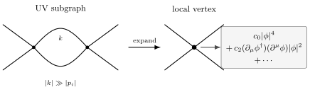
When the loop momentum is much larger than all external momenta, the loop is unresolved by the external fields. Its divergent part collapses to a sum of local operators such as $|\phi|^4$, derivative corrections, and higher-dimensional terms.

This is the conceptual core of perturbative renormalization. A divergent subgraph cannot demand an arbitrary nonlocal modification of the theory. It can only demand that the coefficients of local terms in the Lagrangian be adjusted. At higher loops, this locality statement applies to the remaining overall divergence after divergent proper subgraphs have been subtracted; an unsubtracted diagram can contain nonlocal subdivergent terms.

Effective Lagrangians and changing the cutoff

Let $S_\Lambda$ denote an action defined with modes up to a cutoff $\Lambda$. Split a field into slow and fast modes,

$$\phi=\phi_{<}+\phi_{>},$$

where $\phi_{<}$ contains Euclidean momenta $|p|<\Lambda'$ and $\phi_{>}$ contains the shell $\Lambda'<|p|<\Lambda$. With a finite regulator and a convergent Euclidean measure, the exact Wilsonian action is defined, up to a field-independent normalization, by

$$e^{-S_{E,\Lambda'}[\phi_{<}]} =\int_{\Lambda'<|p|<\Lambda}\mathcal D\phi_{>}\, e^{-S_{E,\Lambda}[\phi_{<}+\phi_{>}]}.$$

The modes in the shell are not thrown away. Their effects are transferred into the lower-cutoff action, which generally contains momentum-dependent interaction kernels. Retaining all those kernels is part of the exact definition.

For example, start from $S_{E,\mathrm{int}}=\lambda\int\phi^4/4!$ with $\lambda>0$. The mixed term $V=(\lambda/4)\int\phi_<^2\phi_>^2$ contributes $-\tfrac12\langle V^2\rangle_{>,c}$ to the action. Wick’s identity $\langle\phi_>^2(x)\phi_>^2(y)\rangle_c=2G_>(x-y)^2$ therefore gives the bilocal term

$$\delta S_E^{(2)}\supset -\frac{\lambda^2}{16}\int d^4x\,d^4y\, \phi_<^2(x)G_>(x-y)^2\phi_<^2(y),$$

where $G_>$ is the regulated fast-mode covariance. It is not a contact interaction before a low-momentum expansion; the canonical shell calculation develops this example.

A local derivative expansion requires external momentum combinations $Q\ll\Lambda'$ and appropriate regularity of the kernels near $Q=0$. With that control, a finite truncation can be written

$$S_{E,\Lambda'}[\phi] \simeq\int d^4x\sum_{i\in\mathrm{retained}} g_i(\Lambda')\,\mathcal O_i(x),$$

with a remainder estimated in that momentum regime. Smooth cutoff choices facilitate such a quasi-local expansion; a sharp shell can introduce nonanalytic dependence at its boundary, so analyticity must not be assumed merely from the picture of a shell. The whole retained band $|p|<\Lambda'$ is not parametrically separated from the eliminated modes. Wilson and Kogut keep momentum-dependent vertices before explicitly making a local approximation: Wilson and Kogut 1974, § 4, pp. 103–106, Eqs. 4.9 and 4.19–4.26.

Within a controlled local truncation, one may equivalently write

$$\mathcal L_{\Lambda'} =\mathcal L_\Lambda+ \sum_i C_i(\Lambda,\Lambda')\mathcal O_i.$$

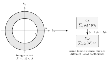
Lowering the cutoff from $\Lambda$ to $\Lambda'$ integrates out a shell of high-momentum modes. The local-coefficient description on the right applies for $Q\ll\Lambda'$ when the derivative expansion is controlled. The exact action retains momentum-dependent kernels. This momentum-plane section and the coefficient flow are schematic.

The operators $\mathcal O_i$ are constrained by the symmetries of the theory. In a scalar theory with $\phi\to -\phi$, the allowed operators include $\phi^2$, $(\partial\phi)^2$, $\phi^4$, $\phi^6$, and so on. In scalar QED, the gauge-invariant sector must obey the Ward identities, with gauge fixing and any regulator-induced breaking treated separately. Renormalization combines dimensional analysis, locality and symmetry.

For a small shell, write

$$\Lambda'=\Lambda e^{-d\ell}.$$

The couplings obey differential flow equations

$${dg_i\over d\ell}=B_i(g_1,g_2,\ldots).$$

This is the Wilsonian renormalization group. The word “group” is historical: lowering the cutoff from $\Lambda$ to $\Lambda''$ can be done directly or by passing through an intermediate cutoff $\Lambda'$, and the result is the same after the appropriate rescaling and coupling redefinition. Strict coarse graining discards short-distance information and is therefore naturally a semigroup rather than an invertible group; the familiar name emphasizes the composition law of successive scale transformations.

Near the Gaussian fixed point, the leading part of this flow is dimensional. If $\mathcal O_i$ has engineering dimension $\Delta_i$ in four spacetime dimensions, then

$$[g_i]=4-\Delta_i.$$

After making couplings dimensionless, the linearized flow contains

$${d\bar g_i\over d\ell}=(4-\Delta_i)\bar g_i+\cdots$$

for the convention in which $\ell$ increases toward the infrared. Thus relevant operators with $\Delta_i<4$ grow under coarse graining, irrelevant operators with $\Delta_i>4$ shrink, and marginal operators require loop corrections to decide their fate.

This Wilsonian equation uses $\ell$ increasing toward the infrared. The beta functions later in the page use $\mu\,d/d\mu$, which increases toward the ultraviolet. The same physical flow can therefore look sign-reversed if one switches scale variables without saying so.

Scalar QED and the running set of couplings

A compact example that contains both matter self-interactions and gauge interactions is scalar QED. Its gauge-invariant Lagrangian is

$$\mathcal L =-{1\over4}F_{\mu\nu}F^{\mu\nu} +|D_\mu\phi|^2 -m^2|\phi|^2 -\lambda |\phi|^4,$$

with

$$D_\mu=\partial_\mu-ieA_\mu.$$

Here $\phi$ is taken to have charge $+e$, so $\phi\mapsto e^{ie\alpha}\phi$ and $A_\mu\mapsto A_\mu+\partial_\mu\alpha$. The conjugate field has the opposite charge. We work perturbatively in the unbroken phase of this anomaly-free theory. A regulator that preserves the vector Ward identities keeps the symmetry constraints manifest. A hard cutoff can break them and require local symmetry-restoring counterterms; the identities constrain the complete renormalized sum, not every separate graph or intermediate term. See the canonical treatment of regulator breaking.

A Wilsonian action at a sliding cutoff $\Lambda$ has coefficients

$$e(\Lambda), \qquad m^2(\Lambda), \qquad \lambda(\Lambda), \qquad Z_\phi(\Lambda), \qquad Z_A(\Lambda),$$

and, in a symmetry-preserving description, an infinite tower of higher-dimensional gauge-invariant operators. Their local expansion is subject to the low-momentum restrictions already stated.

When the cutoff changes,

$$\Lambda\longrightarrow\Lambda',$$

these coefficients flow:

$$e(\Lambda)\longrightarrow e(\Lambda'), \qquad m^2(\Lambda)\longrightarrow m^2(\Lambda'), \qquad \lambda(\Lambda)\longrightarrow \lambda(\Lambda'), \qquad Z_\phi(\Lambda)\longrightarrow Z_\phi(\Lambda'), \qquad Z_A(\Lambda)\longrightarrow Z_A(\Lambda').$$

These are Wilsonian couplings along a trajectory of effective actions, not measured constants. It is useful to distinguish this from regulator language. If $\Lambda$ is a regulator that will be removed, the bare parameters $e_0(\Lambda)$, $m_0^2(\Lambda)$, and $\lambda_0(\Lambda)$ are tuned as the regulator changes so that observables stay fixed. If $\Lambda$ is a sliding Wilsonian resolution, the functions $g_i(\Lambda)$ record the effects of modes already integrated out. In a renormalized description, one instead varies $\mu$ while holding the bare theory fixed. All three descriptions encode the same scale dependence, but the quantities held fixed are different.

In the final gauge-invariant sector of scalar QED, the possible running terms are constrained by the restored Ward identities. For example,

$$F_{\mu\nu}F^{\mu\nu}, \qquad |D_\mu\phi|^2, \qquad |\phi|^2, \qquad |\phi|^4$$

are allowed local operators, while

$$A_\mu A^\mu$$

is not an allowed independent photon-mass counterterm in that sector. Renormalization can change the photon kinetic term, charge, scalar mass, scalar field normalization, and scalar self-coupling while preserving the massless photon of the perturbative unbroken phase. Higgs mass generation in a different phase is not the addition of an explicit gauge-breaking photon-mass term.

The two marginal couplings $e$ and $\lambda$ generally run together:

$$\mu {de\over d\mu}=\beta_e(e,\lambda), \qquad \mu {d\lambda\over d\mu}=\beta_\lambda(e,\lambda).$$

At weak coupling the schematic form is

$$\beta_e=b_e e^3+\cdots,$$

and

$$\beta_\lambda =b_{\lambda\lambda}\lambda^2 +b_{e\lambda}e^2\lambda +b_{ee}e^4+\cdots .$$

The numerical coefficients depend on the normalization of $\lambda$ and on the charged matter content. With the same tree-level definitions of the couplings, the one-loop coefficients are unchanged by finite perturbative scheme redefinitions that begin beyond tree level; higher-loop coefficients can be scheme dependent. The main lesson does not depend on those details: marginal couplings can acquire logarithmic scale dependence, and in a theory with several marginal couplings the RG flow is a vector field on coupling space. Never compare quoted coefficients without first checking the operator normalization, matter content, loop order, and scheme.

Renormalized couplings and logarithms

For a single-coupling example, take real scalar theory in four dimensions with interaction $-\lambda\phi^4/4!$. Define $\lambda(\mu)$ by an off-shell four-point subtraction condition at a nonexceptional Euclidean momentum scale $\mu$. Scale all external momenta together, keeping their ratios fixed. Use the massless theory, or the leading high-energy approximation with both $q$ and $\mu$ much larger than the scalar mass and with mass-suppressed corrections omitted. This avoids importing threshold behavior into a constant-coefficient logarithm.

The subtraction condition defines a renormalization scheme; relating its coupling to measured scattering data requires a calculation. At one loop, applying the same condition at scale $q$ gives

$$\lambda(q) =\lambda(\mu)+b\lambda(\mu)^2\log{q\over\mu}+O(\lambda^3),$$

where $b$ is a one-loop coefficient in the chosen convention. This is the simplest appearance of a running coupling.

Holding the bare theory fixed and changing the subtraction scale gives the same information in differential form. The expression can be written in a form that resums the leading logarithms generated by repeated one-loop insertions:

$$\lambda(q) ={\lambda(\mu) \over 1-b\lambda(\mu)\log(q/\mu)} +O(\text{nonleading logs}).$$

Expanding the denominator gives

$$\lambda(q) =\lambda(\mu) +b\lambda(\mu)^2\log{q\over\mu} +b^2\lambda(\mu)^3\log^2{q\over\mu} +\cdots .$$

Thus the one-loop beta function does more than reproduce the one-loop logarithm. It predicts an infinite tower of leading logarithms.

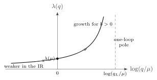
For $\beta(\lambda)=b\lambda^2$ with $b>0$ and a positive initial coupling, the one-loop solution grows toward the ultraviolet and decreases toward the infrared. The horizontal variable measures a logarithmic scale ratio. The schematic curve applies while the running coupling remains perturbative.

The corresponding beta function is

$$\beta_\lambda(\lambda) =\mu{d\lambda\over d\mu} =b\lambda^2+O(\lambda^3).$$

At this order the solution is

$${1\over\lambda(\mu)} ={1\over\lambda(\mu_0)}-b\log{\mu\over\mu_0},$$

or

$$\lambda(\mu) ={\lambda(\mu_0) \over 1-b\lambda(\mu_0)\log(\mu/\mu_0)}.$$

For $b>0$ and $\lambda(\mu_0)>0$, this solution has an ultraviolet pole at

$$\mu_L=\mu_0\exp\left[{1\over b\lambda(\mu_0)}\right].$$

This is a Landau pole in the perturbative running. It should not be overinterpreted as an exact singularity of nature. It says that the weak-coupling description cannot be extrapolated indefinitely beyond that scale.

Callan–Symanzik equation

The same idea can be stated without a literal cutoff. Let $G_R^{(n)}(p_i;\mu,g,m)$ be a renormalized $n$-point function and write the bare field as $\phi_0=Z_\phi^{1/2}\phi_R$. We fix the anomalous-dimension signs by

$$\gamma_\phi ={1\over2} \left.\mu{d\log Z_\phi\over d\mu}\right|_{\mathrm{bare}}, \qquad \gamma_m =-\left.{\mu\over m}{dm\over d\mu}\right|_{\mathrm{bare}}.$$

Equivalently, in the site’s mass-squared notation,

$$\gamma_{m^2}=2\gamma_m, \qquad -\gamma_{m^2}m^2{\partial\over\partial m^2} =-\gamma_m m{\partial\over\partial m}.$$

The scale $\mu$ is arbitrary; it was introduced to define the renormalized parameters. The bare theory does not know about this arbitrary choice. With the beta function and both anomalous dimensions evaluated at fixed bare data, the renormalized correlator satisfies

$$\left( \mu{\partial\over\partial\mu} +\beta_g{\partial\over\partial g} -\gamma_m m{\partial\over\partial m} +n\gamma_\phi \right)G_R^{(n)}(p_i;\mu,g,m)=0,$$

This is the Callan–Symanzik equation in the sign convention just defined.

For an amplitude dominated by a single external scale $q$, the equation says that large logarithms of $q/\mu$ can be avoided by choosing

$$\mu\sim q.$$

Then the amplitude is computed using the coupling appropriate to the momentum flowing through the process:

$$g\to g(q).$$

This is the precise meaning of the phrase “the coupling runs.” It is not that the fundamental rules change from place to place. It is that the best local parameters for a coarse-grained description depend on the scale at which the theory is probed.

Positive and negative beta functions

The sign of the leading beta function controls the qualitative physics. If

$$\beta(\lambda)=+b\lambda^2, \qquad b>0,$$

then the coupling grows toward the ultraviolet. QED has this qualitative behavior: charged matter screens electric charge at long distances, so the effective charge increases at shorter distances. Perturbation theory eventually predicts a Landau pole far outside the domain where ordinary QED is expected to be complete.

If instead a gauge coupling satisfies

$$\beta(g)=-b_0g^3+O(g^5), \qquad b_0>0,$$

then

$${1\over g^2(\mu)} ={1\over g^2(\mu_0)}+2b_0\log{\mu\over\mu_0}.$$

The coupling decreases at short distances. This is asymptotic freedom. The one-loop solution grows toward the infrared, but extrapolating it beyond weak coupling does not determine the infrared endpoint. Higher-order terms can instead produce an interacting infrared fixed point, as the canonical two-term flow demonstrates. Strong infrared coupling or confinement requires further information about the theory.

For an asymptotically free theory, the running can be written as

$$g^2(\mu)={1\over 2b_0\log(\mu/\Lambda_{\mathrm{dyn}})},$$

where

$$\Lambda_{\mathrm{dyn}} =\mu\exp\left[-{1\over 2b_0g^2(\mu)}\right].$$

This is dimensional transmutation. A dimensionless coupling is traded for a dimensionful scale. The classical Lagrangian may have no mass scale, but the quantum theory generates one through logarithmic running.

This course stops at the doorway of that idea. In the next course, the same logic becomes central in non-Abelian gauge theory, sigma models, confinement, instantons, and the modern Wilsonian view of QFT.

Example: resumming a leading logarithm

Return to the real scalar theory and fixed nonexceptional Euclidean momentum ratios specified above, in the massless or stated high-energy regime. Let $\Gamma^{(4)}$ denote its renormalized 1PI four-point vertex coefficient with the overall Feynman factor $i$ omitted, so its tree value is $-\lambda$. This off-shell vertex is not itself an on-shell scattering amplitude. The field anomalous dimension begins at two loops, $\gamma_\phi=O(\lambda^2)$, and affects subleading logarithms here. The canonical scalar four-point calculation keeps that contribution explicitly.

With the finite part fixed by the subtraction condition, the one-loop vertex has the leading-logarithmic form

$$\Gamma^{(4)}(q) =-\lambda(\mu) \left[1+b\lambda(\mu)\log{q\over\mu}+O(\lambda^2)\right].$$

The renormalization group says that, to leading-log accuracy, this is improved by replacing $\lambda(\mu)$ with the running coupling $\lambda(q)$:

$$\Gamma^{(4)}(q)\simeq -\lambda(q).$$

Using the one-loop solution,

$$\Gamma^{(4)}(q) \simeq -{\lambda(\mu)\over 1-b\lambda(\mu)\log(q/\mu)}.$$

Expanding the denominator reproduces the leading logarithms:

$$\Gamma^{(4)}(q) \simeq -\lambda(\mu) \left[1+b\lambda(\mu)\log{q\over\mu} +b^2\lambda(\mu)^2\log^2{q\over\mu}+\cdots\right].$$

A finite-order loop calculation gives the first few logarithms. The beta function organizes the infinite tower.

Summary

Renormalization absorbs ultraviolet sensitivity into local operators. With ultraviolet and infrared regularization in place, loop contributions are finite at a finite cutoff; their ultraviolet parts contain local cutoff-dependent terms that can diverge when the cutoff is removed. At higher loops, divergent subgraphs must first be subtracted. A Wilsonian action retains more general momentum-dependent kernels, whose local derivative expansion has the stated low-momentum scope. Changing the cutoff changes the coefficients while preserving the long-distance observables being matched.

For relevant operators, renormalization changes masses and vacuum energies. For marginal operators, the ultraviolet sensitivity is logarithmic. These logarithms become beta functions, and beta functions define running couplings. The one-loop equation $\beta(\lambda)=b\lambda^2$ resums powers of $\lambda\log(q/\mu)$; the sign of $b$ decides whether the coupling grows or decreases toward short distances.

The deepest lesson is that a quantum field theory is not defined only by a Lagrangian written at one scale. It is defined by a trajectory in the space of local actions. Symmetry restricts the allowed trajectory; locality makes the trajectory possible; logarithms make it visible.

Common pitfalls

Do not call every cutoff-dependent quantity unphysical. Bare parameters are cutoff dependent precisely so that physical quantities are cutoff independent.

Do not confuse the cutoff $\Lambda$ with the renormalization scale $\mu$. The cutoff is a regulator or Wilsonian resolution scale. The renormalization scale is a convention used to define finite couplings. In Wilsonian language they are related, but not identical; in minimal subtraction $\mu$ can appear even after the regulator has been removed.

Do not treat a Landau pole as an exact physical singularity unless the approximations are under control. It usually signals that the weak-coupling description has reached the edge of its validity.

Do not forget that couplings mix. In a theory with several marginal operators, the beta function is a vector field on coupling space, not a single number. Scalar QED already shows this: $e$ and $\lambda$ cannot be understood as completely independent one-coupling problems once loops are included.

Do not compare RG signs without checking the direction of the flow parameter. Wilsonian coarse graining often uses a variable that increases toward the infrared, while $\mu d/d\mu$ increases toward the ultraviolet.

Do not impose a Ward identity on one selected graph or confuse regulator breaking with a physical photon mass. The complete renormalized result must satisfy the symmetry identities; a gauge-breaking regulator may require local restoring terms before that test passes.

Exercises

Exercise 1 — Solving a one-loop beta function

Let

$$\mu{d\lambda\over d\mu}=b\lambda^2, \qquad b>0.$$

For $\lambda(\mu_0)>0$, solve for $\lambda(\mu)$ and find the scale where the one-loop solution has an ultraviolet pole.

Solution

Separate variables:

$${d\lambda\over\lambda^2}=b{d\mu\over\mu}=b\,d\log\mu.$$

Integrating from $\mu_0$ to $\mu$ gives

$$-{1\over\lambda(\mu)}+{1\over\lambda(\mu_0)} =b\log{\mu\over\mu_0}.$$

Thus

$${1\over\lambda(\mu)} ={1\over\lambda(\mu_0)}-b\log{\mu\over\mu_0},$$

or

$$\lambda(\mu) ={\lambda(\mu_0)\over 1-b\lambda(\mu_0)\log(\mu/\mu_0)}.$$

The denominator vanishes at

$$\mu_L=\mu_0\exp\left[{1\over b\lambda(\mu_0)}\right].$$

This is the one-loop Landau-pole scale.

Exercise 2 — A negative beta function and dimensional transmutation

Let

$$\mu{dg\over d\mu}=-b_0g^3, \qquad b_0>0.$$

For $g(\mu_0)>0$, solve the equation on its weak-coupling branch and show how a dimensionful scale $\Lambda_{\mathrm{dyn}}$ appears.

Solution

It is easiest to differentiate $1/g^2$:

$$\mu{d\over d\mu}{1\over g^2} =-{2\over g^3}\mu{dg\over d\mu} =2b_0.$$

Thus

$${1\over g^2(\mu)} ={1\over g^2(\mu_0)} +2b_0\log{\mu\over\mu_0}.$$

Define $\Lambda_{\mathrm{dyn}}$ by absorbing the integration constant:

$${1\over g^2(\mu)} =2b_0\log{\mu\over\Lambda_{\mathrm{dyn}}}.$$

Solving gives

$$\Lambda_{\mathrm{dyn}} =\mu\exp\left[-{1\over 2b_0g^2(\mu)}\right].$$

The dimensionless coupling has been traded for a dimensionful scale. This is dimensional transmutation.

Exercise 3 — Classifying scalar-QED operators

In four spacetime dimensions, classify the following scalar-QED operators as relevant, marginal, or irrelevant by engineering dimension:

$$\phi^\dagger\phi, \qquad (D_\mu\phi)^\dagger D^\mu\phi, \qquad F_{\mu\nu}F^{\mu\nu}, \qquad (\phi^\dagger\phi)^2, \qquad (\phi^\dagger\phi)^3, \qquad (\phi^\dagger\phi)F_{\mu\nu}F^{\mu\nu}.$$

Use $[\phi]=1$, $[A_\mu]=1$, $[D_\mu]=1$, and $[F_{\mu\nu}]=2$.

Solution

The dimensions are

$$[\phi^\dagger\phi]=2,$$

so $\phi^\dagger\phi$ is relevant.

Next,

$$[(D_\mu\phi)^\dagger D^\mu\phi]=2+2[\phi]=4,$$

so the scalar kinetic term is marginal by engineering dimension.

Also,

$$[F_{\mu\nu}F^{\mu\nu}]=4,$$

so the gauge kinetic term is marginal.

For the quartic interaction,

$$[(\phi^\dagger\phi)^2]=4,$$

so it is marginal in four dimensions.

For the sextic interaction,

$$[(\phi^\dagger\phi)^3]=6,$$

so it is irrelevant.

Finally,

$$[(\phi^\dagger\phi)F_{\mu\nu}F^{\mu\nu}]=2+4=6,$$

so this operator is also irrelevant and appears with a coefficient of order $1/\Lambda^2$ in a four-dimensional effective field theory.

Exercise 4 — A logarithmic shell integral

Evaluate the Euclidean shell integral

$$I(\Lambda,\Lambda')= \int_{\Lambda'<|k|<\Lambda}{d^4k\over(2\pi)^4}\,{1\over k^4}.$$

Solution

The area of the unit three-sphere is $\Omega_3=2\pi^2$. Therefore

$$I(\Lambda,\Lambda') ={2\pi^2\over(2\pi)^4} \int_{\Lambda'}^\Lambda dk\,{k^3\over k^4}.$$

Thus

$$I(\Lambda,\Lambda') ={1\over8\pi^2}\int_{\Lambda'}^\Lambda {dk\over k} ={1\over8\pi^2}\log{\Lambda\over\Lambda'}.$$

This is the basic logarithm produced by a four-dimensional loop whose ultraviolet integrand behaves as $1/k^4$.

References

• Wilson, Kenneth G., and John Kogut. “The Renormalization Group and the ε Expansion.” Physics Reports 12, no. 2 (1974): 75–199. DOI.

Further reading

• Coleman, Sidney. Lectures of Sidney Coleman on Quantum Field Theory. Edited by Bryan Gin-ge Chen, David Derbes, David Griffiths, Brian Hill, Richard Sohn, and Yuan-Sen Ting. World Scientific, 2019. DOI.
• Polyakov, A. M. Gauge Fields and Strings. Harwood Academic Publishers, 1987. DOI and open-access edition.
• Srednicki, Mark. Quantum Field Theory. Cambridge University Press, 2007. DOI.
• Weinberg, Steven. The Quantum Theory of Fields, Volume I: Foundations. Cambridge University Press, 1995. DOI.
• Weinberg, Steven. The Quantum Theory of Fields, Volume II: Modern Applications. Cambridge University Press, 1996. DOI.
• Zee, A. Quantum Field Theory in a Nutshell. 2nd ed. Princeton University Press, 2010. Publisher.