

Proper Time, Determinants, and Thermal Traces
The previous page used vacuum polarization to motivate the running charge and introduced the physical image of closed charged worldlines. This page makes that image into a calculational tool. The basic object is no longer a single Feynman diagram written in momentum space, but a functional determinant written as a trace of an evolution operator.
The bridge is Schwinger’s proper-time representation:
Here is not physical time. It is a Laplace-transform parameter that probes the spectrum of the Euclidean operator . Small sees large eigenvalues and therefore short distances; large sees low eigenvalues and therefore infrared physics. This is why proper time is so useful for renormalization: ultraviolet divergences become the small- asymptotics of a heat kernel.
The same trace language also explains finite-temperature path integrals. A thermal partition function is
and the trace turns Euclidean time into a circle of circumference . Bosonic variables are periodic, fermionic variables are antiperiodic, and Matsubara frequencies are simply the Fourier modes on that circle. The two themes — determinant traces and thermal traces — are really the same technology used in two different spectral problems.
Required background. Vacuum Polarization and Gauge-Invariant Counterterms fixes the Euclidean gauge-field normalization and scalar-QED determinant sign. Running Charge, Screening, and Antiscreening supplies the closed-worldline interpretation that proper time makes precise below.
A useful reader’s dictionary for this page is:
The notation is similar enough to be dangerous. The parameter regulates a determinant; the parameter is the physical circumference of the Euclidean-time circle.
Gaussian integrals and one-loop determinants
Section titled “Gaussian integrals and one-loop determinants”Most formulas on this page are Euclidean. Consider the Laplace-type expression
for a unit-charge complex scalar in a smooth, real background Abelian field. A differential expression alone does not define its spectrum. Choose a self-adjoint realization with compatible boundary conditions, and assume a strictly positive lower spectral bound. For , and the usual covariant domain, supplies that bound; an arbitrary need not. A finite-volume heat trace must be trace class. The constant-field formulas below instead use the thermodynamic trace per unit volume. They are not exact hard-wall finite-box spectra.
Zero modes must be removed explicitly or given an infrared regulator; negative modes require a separate contour prescription. A small-proper-time cutoff resolves neither issue. Heat Kernels, Zeta Functions, and Spectral Determinants develops the operator and boundary hypotheses. The operator dimension inside a logarithm is fixed by a reference scale , but field-independent constants are suppressed unless they matter.
A real bosonic Gaussian contributes
a complex bosonic Gaussian contributes
and a Grassmann Gaussian contributes with the opposite sign,
These signs are the most common source of mistakes in this subject.
The sign convention can be checked by remembering that . A complex boson gives , hence . A Grassmann field gives , hence .
Start with an ordinary finite-dimensional Gaussian integral. If is a real, symmetric, positive matrix, then
For complex variables,
For Grassmann variables,
The infinite-dimensional version requires a regulator and counterterms. The determinant identities below first mean finite-dimensional Gaussian algebra; later we specify a proper-time cutoff separately. Consider a complex scalar field in a fixed Euclidean background ,
The matter path integral is
The one-loop effective action is defined by
so
For a real scalar the answer is half as large. For a Dirac fermion,
and the Grassmann integral gives
The trace includes the integral over spacetime, the sum over internal indices, and, for fermions, the trace over spinor indices. Integrating out these Gaussian matter fields is developed in Schwartz 2014, § 33.3, pp. 711–712; the displayed signs here use the Euclidean weight .
For fermions, this first-order determinant may later be squared into a Laplace-type determinant, but that step must be done with care. Squaring gives useful heat-kernel formulas for parity-even terms such as , while possible phases of the determinant carry anomaly information. In these notes, whenever we square a Dirac operator we state explicitly which parity-even part is being extracted.
Two comments are worth making immediately. First, a determinant is only meaningful after specifying a regulator and a normalization. Ratios such as
are better behaved than either determinant separately, because field-independent vacuum-volume terms cancel. Second, the determinant knows about all one-loop diagrams with any number of external background-field insertions. Expanding
gives, in a finite regulator with and for sufficiently small ,
and therefore
This expansion counts powers of , which need not equal powers of the background. For the scalar operator, direct multiplication of gives
Thus the complete term of order is
The first term is the two-photon seagull and the second is the bubble with two one-photon vertices. Both are required for the scalar vacuum polarization. This is the same nonlinear source dependence as in Current Sources and Generating Functionals. At order , two seagulls and mixed one- and two-photon vertices also contribute; the next lesson groups them explicitly. Charge conjugation cancels odd background powers in the vectorlike Abelian vacuum considered here. It does not mean each odd power of vanishes separately.
Proper time and the heat kernel
Section titled “Proper time and the heat kernel”Suppose has positive eigenvalues . Then
The logarithm can be represented by a proper-time integral. A useful subtracted identity is
which follows by differentiating with respect to and fixing the value at . A proper-time prescription for a field-theory determinant is
where
is a short-proper-time cutoff. This is a definition at finite , not the ordinary logarithm of each eigenvalue plus an eigenvalue-independent constant. Its derivative with respect to an eigenvalue is . Counterterms must be added before removing the UV cutoff. In the following finite-cutoff formulas, denotes this regulated matter contribution before those counterterms. After subtracting the vacuum term,
The kernel of is the heat kernel,
It obeys
The trace is obtained by closing the endpoints:
The lower-case trace is over finite-dimensional indices such as spin, flavor, or gauge representation indices.
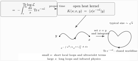
Proper time turns the determinant into an open heat kernel. Taking the trace identifies the endpoints and produces a closed charged worldline. Short loops of size control ultraviolet terms; long loops probe infrared physics.
The ultraviolet structure is local because it comes from the short- expansion of the heat kernel. This is one of the cleanest ways to see why ultraviolet divergences are removable by local counterterms: at very small , the heat kernel samples only an infinitesimal neighborhood of the point . For a Laplace-type operator in flat space,
The coefficients are local functions of the background fields and their derivatives. This is the smooth interior, or boundary-free, expansion; a trace with a boundary generally also contains boundary terms with half-integer powers of . In , the interior terms , , and multiply respectively , , and in . Thus gives a quartic divergence, a quadratic divergence, and a logarithmic divergence. Gauge coupling renormalization lives in the coefficient.
For the minimal Abelian scalar operator
the first gauge-field term is
The sign is important. The heat trace itself decreases in a weak magnetic field; this is the orbital diamagnetic sign. But the scalar effective action has an overall minus sign in the proper-time integral, so the induced Maxwell term is positive. The distinction between the sign inside the heat kernel and the sign in the effective action is a small bookkeeping point that becomes physically important on the next two pages.
In this gives
Keeping only the logarithmic divergence,
If the Maxwell action is written as
then matching requires multiplying the coefficient of by . Thus one complex scalar shifts
which is the scalar QED coefficient used earlier.
Heat kernels as charged worldlines
Section titled “Heat kernels as charged worldlines”Proper time converts the spectral operator into a particle path integral. This is the precise bridge between the vacuum-polarization loop of the previous pages and the closed-worldline picture in the manuscript. Begin with the background-field propagator
For a positive Euclidean operator,
so
The open heat kernel has the configuration-space representation
The sign of the Wilson phase follows directly from . Indeed,
and integrating the first-order momentum path integral produces . Under
the open Wilson phase supplies exactly the endpoint phases required for to transform covariantly.
Taking the trace identifies the endpoints and turns the open trajectory into a closed loop:
The endpoint phases now cancel, so each closed path is weighted by a gauge-invariant Wilson loop. Substituting this trace into the proper-time determinant sums closed charged trajectories of every proper duration . Typical loops have size : short loops generate the local ultraviolet expansion, while long loops probe infrared propagation.
For a slowly varying field, the Wilson loop measures the flux through the trajectory. Expanding that flux gives local powers of ; averaging over loop orientation removes the term linear in and leaves as the first Abelian contribution. This is the worldline explanation of why the same determinant reproduces the transverse vacuum-polarization term.
Proper-time closure and thermal closure must nevertheless be distinguished. In a determinant, is integrated from zero to infinity. In a thermal trace, the Euclidean-time circumference is fixed by the temperature. The paths are closed in both cases, but the parameters play different physical roles.
Time ordering inside an operator trace
Section titled “Time ordering inside an operator trace”The notation looks innocent, but when is built from noncommuting operators the trace is not a classical phase-space integral. The distinction is already visible in a finite-dimensional Hilbert space.
For two noncommuting operators and , one cannot write
Instead, introduce
Duhamel’s formula gives
where orders larger to the left. Expanding to first order reproduces
This is the operator origin of time-ordered perturbation theory. In a trace, cyclicity identifies the beginning and end of the interval, so insertions live on a circle.
Time ordering also produces contact terms. If and are Heisenberg operators with
then
Differentiating gives
At equal time the commutator is , so
in a state normalized so that . This delta function is the tiny but crucial trace of noncommutativity. Any path-integral derivation that replaces operators by ordinary functions must reproduce these contact terms through its discretization prescription.
First-order path integrals and closed trajectories
Section titled “First-order path integrals and closed trajectories”The thermal trace of a quantum-mechanical Hamiltonian is
Take flat Cartesian canonical coordinates, a self-adjoint Hamiltonian bounded below, and a trace-class (or a declared bulk trace density). Operator ordering is additional data. For the smooth magnetic Schrödinger Hamiltonian used below, choose its Weyl symbol and midpoint time slicing. Insert complete sets of and eigenstates at many intermediate Euclidean times. Using
up to the standard normalization, the time-sliced definition in one dimension is
The limit presumes the usual convergent short-time construction for this Hamiltonian; this is not a rule for an arbitrary unbounded composite operator. The Weyl-to-midpoint step is explained in Bastianelli, Schalm and van Nieuwenhuizen 1998, Eq. (2), PDF p. 3. Its continuum notation is
The trace is responsible for the periodic boundary condition. In several dimensions this becomes
The term is the Euclidean version of the symplectic one-form. It encodes the canonical structure; the symbol and time slicing specify ordering. For example, if , direct use of gives
Here is the average of the six distinct orderings of two ‘s and two ‘s. Thus the Weyl symbol of is , not just the square of the symbol of . The symplectic term alone cannot recover this missing constant. In the following schematic, read the midpoint definition before its canonical contact check.
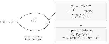
The thermal trace closes the coordinate path. The first-order weight uses with midpoint time slicing; encodes canonical structure but does not choose the ordering of a composite Hamiltonian. The contact identity uses normalized thermal expectation values and Euclidean time ordering, away from the circle seam. Schematic, not a sampled trajectory.
For a positively charged unit particle with , the function
is the Weyl symbol of . The momentum integral is Gaussian. Completing the square at each midpoint gives the second-order path integral
The vector potential appears through the same Wilson phase as in the relativistic heat kernel. Its line integral is defined by the midpoint, or Stratonovich, limit for the generally nondifferentiable paths. A particle of charge is obtained by replacing with ; changing the sign of complex-conjugates the phase but leaves the magnetic spectrum unchanged.
The classical partition function would be
The quantum trace reduces to this expression only in an appropriate semiclassical or high-temperature limit. In the full quantum trace, nonzero Fourier modes contribute quantum fluctuations, while the chosen symbol and time slicing preserve operator ordering.
For a bosonic coordinate on the thermal circle,
When is small, the nonzero modes have large frequencies. In many problems the zero mode dominates the leading classical thermodynamics, while the nonzero modes produce quantum corrections.
Thermal circles and Matsubara determinants
Section titled “Thermal circles and Matsubara determinants”In quantum field theory the same trace gives the finite-temperature Euclidean path integral,
Euclidean time is compact:
Bosons are periodic,
while fermions are antiperiodic,
The minus sign for fermions is required by the trace over fermionic states and the Grassmann nature of fermionic coherent states. It leads to different Matsubara frequencies:
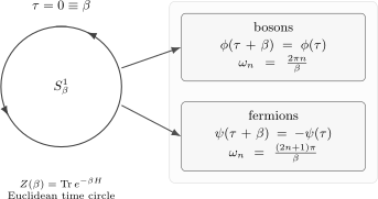
A thermal trace compactifies Euclidean time to a circle of circumference . Bosonic fields are periodic and have frequencies ; fermionic fields are antiperiodic and have frequencies .
The harmonic oscillator is the cleanest check. Its exact thermal trace is
The Euclidean path integral gives the same result as a determinant,
where P means periodic boundary conditions. The eigenvalues are
The infinite product is regulated, but its dependence is fixed by
Thus the determinant knows the oscillator spectrum.
For a free scalar field, each spatial momentum mode is an oscillator with
The one-loop thermal free energy density is therefore
after the usual normalization of the zero-point energy. For a free Dirac fermion the antiperiodic determinant gives the Fermi–Dirac factor
with the appropriate spin and particle–antiparticle degeneracies and with the overall fermionic sign in the free energy.
Landau levels as a trace calculation
Section titled “Landau levels as a trace calculation”A constant magnetic field gives a useful test of all these ideas. Consider a positively charged unit spinless particle moving in two spatial dimensions with and magnetic field . Its Hamiltonian is
The kinetic momenta
satisfy
The sign fixes which linear combination is the raising operator; the spectrum depends only on . For , the energy levels are
and the bulk number of states per unit area in each level is . We write the extensive bulk trace for an area using
This count is exact on a magnetic torus with compatible boundary conditions and quantized flux , . For an ordinary finite region with walls, edge states change the answer. The bulk counting and torus qualification are explained in Tong, undated author chapter, § 1.4.1, Eqs. (1.21)–(1.22), PDF pp. 20–21. In the bulk notation, the one-particle thermal trace is
At high temperature,
The leading term is the classical phase-space answer. The correction is the first orbital quantum correction. The figure shows how equal Landau spacing and the common bulk degeneracy make the sum geometric.
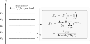
A constant magnetic field gives for unit charge and . Each level has bulk density per unit area, so is a geometric sum in . The levels are exact; the finite set of dots schematically indicates degeneracy. A finite torus requires quantized flux; hard-wall edge corrections are excluded.
The four-dimensional heat kernel in a constant magnetic field is the same bulk calculation with two additional infinite free Euclidean directions. Here denotes the thermodynamic trace density, not the exact trace in an arbitrary finite box. For the scalar operator ,
Expanding for small ,
Since for a purely magnetic field in Euclidean space, this agrees with the heat-kernel coefficient
This is the calculation that the next pages will refine for scalar, spinor, and vector fluctuations in background fields.
A useful diagnostic is that is dimensionless: and . Expanding it organizes powers of the field strength. It is not a derivative expansion: a constant field has no gradients but still contributes at every even field-strength order. In a massive low-energy effective action, a weak-field truncation needs , while a derivative truncation separately needs background variation scales much smaller than .
Summary
Section titled “Summary”A one-loop path integral is a functional determinant. Bosonic fluctuations give inverse determinants in and positive terms in the effective action; fermionic fluctuations give determinants in and negative terms in the effective action.
Schwinger proper time defines the regulated trace logarithm through a heat trace:
The renormalized effective action is obtained only after adding the prescribed counterterms and taking the regulated limit, with the infrared assumptions stated above.
The heat kernel solves a diffusion equation in the auxiliary variable . Its small- expansion is local and controls ultraviolet divergences. In four-dimensional scalar QED, the term in this expansion reproduces the scalar contribution
The open heat kernel is also a charged-particle path integral. With , each path carries . Taking the trace identifies its endpoints, producing a gauge-invariant Wilson loop and the closed-worldline representation of the determinant.
Thermal traces use the same logic with physical Euclidean time compactified to a circle of circumference . Periodic bosonic fields have frequencies , antiperiodic fermionic fields have frequencies , and functional determinants reduce to products over these modes. Landau levels provide an especially concrete example: a magnetic field discretizes transverse motion, and the trace becomes a weighted sum over oscillator levels.
Common pitfalls
Section titled “Common pitfalls”Proper time is not thermal Euclidean time. Proper time is a spectral parameter used to represent logarithms and inverse operators. Thermal Euclidean time has physical period .
Determinant powers and signs matter. A real scalar, complex scalar, and Dirac fermion differ by factors of and by an overall sign. These differences produce different one-loop coefficients.
A quantum trace is not automatically a classical phase-space integral. Replacing by requires a justified semiclassical limit. Operator ordering and contact terms otherwise remain.
Thermal boundary conditions determine the spectrum. Periodic versus antiperiodic conditions change bosonic frequencies into fermionic Matsubara frequencies.
The small- expansion is ultraviolet. Large is where zero modes, masslessness, and infrared divergences enter.
The Wilson-phase sign follows the covariant derivative. With , the worldline phase is . Reversing the charge convention reverses this sign without changing the even-in- terms studied here.
Exercises
Section titled “Exercises”Exercise 1: Track Gaussian determinant powers and signs
Section titled “Exercise 1: Track Gaussian determinant powers and signs”Let be a real symmetric positive matrix. Show that real bosons, complex bosons, and Grassmann variables give determinant powers , , and , respectively, in the partition function. Translate these powers into contributions to . Then check the quadratic trace-log formula on the isospectral family , , where is the two-dimensional rotation matrix. Why is keeping only the bubble inconsistent?
Solution
Diagonalize by a unitary or orthogonal transformation. For a real variable,
so real variables give
For a complex variable , the Gaussian has two real components and gives one inverse power of the eigenvalue:
For Grassmann variables,
up to a convention-dependent sign in the measure. Therefore
Since ,
For , expand . Direct multiplication gives
With ,
They cancel, as required by . The bubble alone would give a nonzero response for . This finite isospectral example checks the same cancellation mechanism needed for a gauge transformation of a scalar operator; it is not a model of the full QFT spectrum.
Exercise 2: Prove the subtracted proper-time identity
Section titled “Exercise 2: Prove the subtracted proper-time identity”Prove the subtracted proper-time identity
for .
Solution
Define
Differentiate with respect to :
Thus
At , the integrand vanishes and . Hence
so . Therefore
The subtraction is essential: each exponential integral separately is divergent at small , but their difference is finite.
Exercise 3: Recover the equal-time contact term
Section titled “Exercise 3: Recover the equal-time contact term”Using
show that
when .
Solution
Differentiate the time-ordered product:
and
Since , the delta-function part is
At the support of the delta function, , so this is
The remaining terms are precisely . Taking the expectation value gives the result.
Exercise 4: Reconstruct the oscillator determinant
Section titled “Exercise 4: Reconstruct the oscillator determinant”The periodic operator on a circle of circumference has eigenvalues
Use the product identity
to show that the determinant reproduces the dependence of the harmonic-oscillator partition function.
Solution
Up to an -independent constant,
Factor out the -independent pieces:
Set
The product identity gives
Therefore
A real oscillator has
The normalization fixed by canonical quantization gives
Exercise 5: Sum the Landau-level thermal trace
Section titled “Exercise 5: Sum the Landau-level thermal trace”For a unit-charge spinless particle in two dimensions with and magnetic field , work with the bulk trace density, or with a magnetic torus whose flux obeys . Use the Landau spectrum
and degeneracy to derive
Then expand the answer for .
Solution
The trace is degeneracy times the Boltzmann sum:
The sum is geometric:
Thus
For small ,
With ,
Therefore
The first term is the classical phase-space result; the term is the leading orbital quantum correction.
Exercise 6: Extract the scalar-QED logarithm from the heat kernel
Section titled “Exercise 6: Extract the scalar-QED logarithm from the heat kernel”Use the four-dimensional scalar heat kernel in a constant magnetic field,
to recover the logarithmic scalar-QED correction to .
Solution
Expand the magnetic factor:
The -independent term contributes only to the vacuum energy. The term gives, for a complex scalar,
Thus
The logarithmic part is
Since for this background,
Therefore
Matching to
gives
References
Section titled “References”- Bastianelli, Fiorenzo, Koenraad Schalm, and Peter van Nieuwenhuizen. “Mode Regularization, Time Slicing, Weyl Ordering, and Phase Space Path Integrals for Quantum-Mechanical Nonlinear Sigma Models.” Physical Review D 58 (1998): 044002. DOI. Open PDF, arXiv v1.
- Schwartz, Matthew D. Quantum Field Theory and the Standard Model. Cambridge University Press, 2014. DOI.
- Tong, David. Lectures on the Quantum Hall Effect. University of Cambridge lecture notes, chapter 1, § 1.4.1. Undated chapter PDF, accessed 7 September 2026. Author’s chapter PDF.
Further reading
Section titled “Further reading”- Schwinger, Julian. “On Gauge Invariance and Vacuum Polarization.” Physical Review 82, no. 5 (1951): 664–679.
- Srednicki, Mark. Quantum Field Theory. Cambridge University Press, 2007.
- Weinberg, Steven. The Quantum Theory of Fields, Volume II: Modern Applications. Cambridge University Press, 1996.
- Zee, A. Quantum Field Theory in a Nutshell. 2nd ed. Princeton University Press, 2010.
- Zinn-Justin, Jean. Quantum Field Theory and Critical Phenomena. 4th ed. Oxford University Press, 2002.