Source Functionals in Quantum Mechanics and QFT

The previous page showed that a free path integral is a Gaussian. That observation is more powerful than it first looks. Once a path integral is written as a Gaussian, we do not want to insert $q(t_1)\cdots q(t_n)$ by hand every time we need a correlator. We want a single object whose derivatives generate all time-ordered Green functions.

That object is the source functional. We couple the coordinate $q(t)$, or later the field $\phi(x)$, to an auxiliary classical function $J$. Differentiating with respect to $J$ pulls down insertions of the quantum variable. The source is therefore a bookkeeper for time-ordered correlators. It can also represent a weak external force, but derivatives of the ordinary Feynman functional generate in–out Green functions, not causal response functions. For perturbation theory its main use here is algebraic: it turns the whole hierarchy of correlators into derivatives of one functional.

This page develops the idea first in ordinary quantum mechanics and then in scalar field theory. The same formulas will become the engine of perturbation theory: interactions become functional differential operators acting on the free Gaussian source functional.

The source as a bookkeeper

This course lesson preserves the oscillator-first derivation and its contact-term exercises. The Generating Functional gives the canonical field-theory definitions and domain of validity. Every shorthand Lorentzian path integral below assumes a finite regulator, the Feynman $i0$ boundary value, and vacuum endcaps or long-time projection. Ordinary Feynman source derivatives compute in–out time-ordered correlators; causal real-time response requires an in–in or Schwinger–Keldysh construction.

Source sign and normalized generating functional

In this page the normalized source functional satisfies $Z[0]=1$, and the source is added to the action as $+\int dt\,J(t)q(t)$ or $+\int d^4x\,J(x)\phi(x)$. With this convention,

$$\langle\mathcal T q(t_1)\cdots q(t_n)\rangle =\left.\frac{1}{i^n}\frac{\delta^nZ[J]}{\delta J(t_1)\cdots\delta J(t_n)}\right|_{J=0}.$$

For the harmonic oscillator, the Feynman Green function is denoted $G_F(t-t')=\langle0|\mathcal T q(t)q(t')|0\rangle$ and obeys

$$(\partial_t^2+\omega^2)G_F(t-t')=-i\delta(t-t').$$

For scalar fields, this page also writes $G_F$ when emphasizing the Green-function role; it is the same object denoted $D_F$ in the qft.org convention page.

Three functionals

Keep three objects separate from the beginning. $Z[J]$ generates full correlators, including disconnected products. $W[J]=-i\log Z[J]$ generates connected correlators. The effective action $\Gamma[\varphi]$, introduced later, generates one-particle-irreducible vertices. Many normalization mistakes come from applying a formula for one of these functionals to another.

For a quantum-mechanical coordinate $q(t)$, define

$$Z[J] =\frac{\displaystyle\int\mathcal Dq\, \exp\left(iS[q]+i\int dt\,J(t)q(t)\right)} {\displaystyle\int\mathcal Dq\,e^{iS[q]}}.$$

The denominator normalizes the vacuum functional so that

$$Z[0]=1.$$

A functional derivative with respect to the source pulls down a factor of the coordinate:

$$\frac{\delta}{\delta J(t_1)} \exp\left(i\int dt\,J(t)q(t)\right) =iq(t_1)\exp\left(i\int dt\,J(t)q(t)\right).$$

Therefore

$$\frac{1}{i}\frac{\delta Z[J]}{\delta J(t_1)} =\frac{\displaystyle\int\mathcal Dq\,e^{iS[q]+i\int Jq}q(t_1)} {\displaystyle\int\mathcal Dq\,e^{iS[q]}}.$$

After differentiating $n$ times and setting $J=0$,

$$\boxed{ \langle\mathcal T q(t_1)\cdots q(t_n)\rangle =\left.\frac{1}{i^n}\frac{\delta^n Z[J]} {\delta J(t_1)\cdots\delta J(t_n)}\right|_{J=0}. }$$

The time-ordering symbol is not optional. The real-time path integral with the Feynman $i0$ boundary-value prescription computes vacuum expectation values with Feynman boundary conditions; these are time-ordered correlators. The source $J$ is a classical function, but it generates quantum Green functions.

The normalization in the denominator is equally important. It removes purely vacuum factors before any operator insertions are considered. Later, when interactions are expanded diagrammatically, this same normalization is what cancels vacuum bubbles disconnected from the external fields.

A useful check on the factors of $i$ is the free Gaussian result. If

$$Z_0[J]=\exp\left[-\frac12\int JG_FJ\right],$$

then

$$\left.\frac{1}{i^2}\frac{\delta^2Z_0[J]}{\delta J(t_1)\delta J(t_2)}\right|_{J=0} =G_F(t_1-t_2),$$

because $1/i^2=-1$ and the second derivative of the exponential gives $-G_F$. This one-line check catches most sign errors in Lorentzian source formulas.

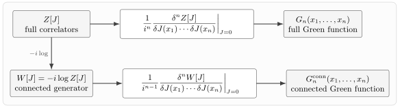
The source $J$ couples linearly to the coordinate or field. Functional derivatives of $Z[J]$ remove source legs and generate time-ordered insertions. Setting $J=0$ after differentiating returns the physical vacuum correlator.

The exact field-theory version uses the selected normalized interacting vacuum $|\Omega\rangle$ and the source-free Heisenberg field $\phi_H$:

$$Z[J] =\langle\Omega|T\exp\left(i\int d^4x\,J(x)\phi_H(x)\right)|\Omega\rangle, \qquad Z[0]=1.$$

With the common regulator and vacuum boundary specified in the canonical note, its shorthand path-integral representation is

$$Z[J] =\frac{\displaystyle\int_{\Omega\to\Omega}\mathcal D\phi\, \exp\left(iS[\phi]+i\int d^4x\,J(x)\phi(x)\right)} {\displaystyle\int_{\Omega\to\Omega}\mathcal D\phi\,e^{iS[\phi]}}.$$

Therefore

$$\boxed{ G_n(x_1, \ldots,x_n) =\langle\Omega|\mathcal T\phi_H(x_1)\cdots\phi_H(x_n)|\Omega\rangle =\left.\frac{1}{i^n}\frac{\delta^nZ[J]} {\delta J(x_1)\cdots\delta J(x_n)}\right|_{J=0}. }$$

This formula is one of the main organizational principles of QFT. Instead of separately defining infinitely many $n$-point functions, we encode them in one object.

A compact dictionary is:

Object	Generated quantity	Derivative rule
$Z[J]$	full time-ordered correlators	$(1/i^n)\delta^n Z/\delta J^n$
$\log Z[J]$	connected correlators	$(1/i^n)\delta^n\log Z/\delta J^n$
$W[J]=-i\log Z[J]$	connected correlators with one fewer explicit $i$	$(1/i^{n-1})\delta^n W/\delta J^n$

The source is set to zero only after differentiating. Setting $J=0$ too early throws away the information the source was introduced to store. Keeping it nonzero temporarily is not a physical deformation of the theory unless we decide to interpret it that way; in perturbation theory it is mainly a control knob that labels insertions.

Functional derivatives from time slicing

The word “functional” can sound more mysterious than it is. It is just the continuum version of differentiating a function of many variables.

Discretize time as

$$t_j=t_i+j\epsilon, \qquad j=0,1,\ldots,N.$$

A path becomes a list of numbers,

$$q(t)\longrightarrow \{q_j\},$$

and a source becomes another list,

$$J(t)\longrightarrow \{J_j\}.$$

The source coupling is approximated by

$$\int dt\,J(t)q(t) \longrightarrow \epsilon\sum_jJ_jq_j.$$

Differentiating with respect to $J_k$ gives

$$\frac{\partial}{\partial J_k} \left(\epsilon\sum_jJ_jq_j\right)=\epsilon q_k.$$

The continuum functional derivative is normalized so that

$$\frac{\delta J(t)}{\delta J(t')}=\delta(t-t'), \qquad \frac{\delta}{\delta J(t)}\int dt'\,J(t')q(t')=q(t).$$

In the time-sliced picture this means roughly

$$\frac{\delta}{\delta J(t_k)}\sim \frac{1}{\epsilon}\frac{\partial}{\partial J_k}.$$

Thus the path integral notation

$$\int\mathcal Dq$$

is not hiding a new kind of calculus. It is the limit of many ordinary integrals, and the functional derivative is the limit of many ordinary partial derivatives with the correct factor of the time-slice spacing.

The Gaussian source functional

Now take the harmonic oscillator with action

$$S_0[q]=\int dt\left(\frac12\dot q^2-\frac12\omega^2q^2\right).$$

After integrating by parts and choosing the Feynman prescription, write

$$S_0[q;J] = -\frac12\int dt\,q(t)Kq(t)+\int dt\,J(t)q(t),$$

where

$$K=\partial_t^2+\omega^2-i0.$$

This definition factors the minus sign out of the quadratic form. On the previous page the Hessian itself was called $K_{\mathrm{Hess}}=-(\partial_t^2+\omega^2)$ and the action was written $+\frac12qK_{\mathrm{Hess}}q$; here $K=-K_{\mathrm{Hess}}$ (with the Feynman boundary value included). The physics and the Green-function equation are unchanged.

The source-dependent stationary configuration satisfies

$$Kq_J(t)=J(t).$$

Since

$$K_tG_F(t-t')=-i\delta(t-t'),$$

the inverse of $K$ is $iG_F$, and therefore

$$q_J(t)=i\int dt'\,G_F(t-t')J(t').$$

Shift the integration variable,

$$q(t)=q_J(t)+\eta(t).$$

The linear term in $\eta$ disappears because $q_J$ solves the sourced equation of motion. The Gaussian determinant from integrating over $\eta$ is independent of $J$ and cancels against the normalization in $Z[0]$. The remaining source dependence is

$$\boxed{ Z_0[J] =\exp\left[-\frac12\int dt\,dt'\, J(t)G_F(t-t')J(t')\right]. }$$

This formula is worth pausing over. The full free theory is contained in the quadratic form $JG_FJ$. The propagator appears because the source shifts the saddle point by the inverse of the quadratic operator.

The minus sign in $Z_0[J]=\exp[-\frac12JG_FJ]$ is not a Euclidean Gaussian sign. It is a Lorentzian source-convention sign. The factor $i$ in $e^{i\int Jq}$ means each insertion is generated by $(1/i)\delta/\delta J$; two such derivatives turn the minus sign back into the positive two-point function $G_F$.

A linear source tilts the quadratic action and moves the saddle from $q=0$ to the sourced configuration $q_J=iG_FJ$. The drawing is a schematic real (or Wick-rotated finite-dimensional) slice of a Lorentzian saddle that can be complex. The normalized free functional keeps only the $J$-dependent saddle contribution; the determinant cancels against $Z_0[0]$.

Check the two-point function directly. Differentiating twice gives

$$\left.\frac{\delta^2Z_0[J]}{\delta J(t_1)\delta J(t_2)}\right|_{J=0} =-G_F(t_1-t_2).$$

Since $1/i^2=-1$,

$$\left.\frac{1}{i^2}\frac{\delta^2Z_0[J]} {\delta J(t_1)\delta J(t_2)}\right|_{J=0} =G_F(t_1-t_2),$$

as required. This minus sign is one of the easiest places to make an error: the Gaussian has $-\frac12JG_FJ$, while each Lorentzian source derivative contributes a factor $1/i$.

Four derivatives give Wick theorem again:

$$\begin{aligned} &\langle0|\mathcal Tq(t_1)q(t_2)q(t_3)q(t_4)|0\rangle \\ &\quad= G_F(t_1-t_2)G_F(t_3-t_4) +G_F(t_1-t_3)G_F(t_2-t_4) \\ &\qquad +G_F(t_1-t_4)G_F(t_2-t_3). \end{aligned}$$

This is the cleanest way to derive free $n$-point functions: differentiate the exponential of a quadratic source functional.

From the oscillator to the scalar field

For a real scalar field, the normalized generating functional is

$$Z[J] =\frac{\displaystyle\int\mathcal D\phi\, \exp\left(iS[\phi]+i\int d^4x\,J(x)\phi(x)\right)} {\displaystyle\int\mathcal D\phi\,e^{iS[\phi]}}.$$

For the free scalar action,

$$S_0[\phi] =\int d^4x\,\frac12\left(\partial_\mu\phi\,\partial^\mu\phi-m^2\phi^2\right),$$

integration by parts gives

$$S_0[\phi;J] =-\frac12\int d^4x\,\phi(x)(\Box+m^2-i0)\phi(x) +\int d^4x\,J(x)\phi(x).$$

The free Feynman propagator satisfies

$$(\Box_x+m^2)G_F(x-y)=-i\delta^{(4)}(x-y),$$

with

$$G_F(x-y) =\int\frac{d^4p}{(2\pi)^4}\, \frac{i\,e^{-ip\cdot(x-y)}}{p^2-m^2+i0}.$$

Repeating the same Gaussian shift gives

$$\boxed{ Z_0[J] =\exp\left[-\frac12\int d^4x\,d^4y\, J(x)G_F(x-y)J(y)\right]. }$$

The field-theory $n$-point functions are therefore

$$\boxed{ \langle0|\mathcal T\phi(x_1)\cdots\phi(x_n)|0\rangle_0 =\left.\frac{1}{i^n}\frac{\delta^nZ_0[J]} {\delta J(x_1)\cdots\delta J(x_n)}\right|_{J=0}. }$$

The subscript $0$ reminds us that this is the free theory. Interactions change $Z[J]$, but the Gaussian $Z_0[J]$ remains the basic object around which perturbation theory is built.

Connected functions and vacuum normalization

The functional $Z[J]$ generates full correlators, including disconnected products. The logarithm removes disconnected pieces. With Lorentzian conventions we write

$$Z[J]=e^{iW[J]}, \qquad W[J]=-i\log Z[J].$$

Connected correlators are the parts that do not factor into independent lower-point experiments. They are also the parts represented by connected diagrams in perturbation theory, after the vacuum normalization has removed vacuum bubbles.

Then connected correlators are generated by

$$\boxed{ G_n^{\mathrm{conn}}(x_1,\ldots,x_n) =\left.\frac{1}{i^{n-1}}\frac{\delta^nW[J]} {\delta J(x_1)\cdots\delta J(x_n)}\right|_{J=0}. }$$

Equivalently,

$$G_n^{\mathrm{conn}}(x_1,\ldots,x_n) =\left.\frac{1}{i^n}\frac{\delta^n\log Z[J]} {\delta J(x_1)\cdots\delta J(x_n)}\right|_{J=0}.$$

For the free scalar field,

$$\log Z_0[J] =-\frac12\int JG_FJ.$$

Therefore $\log Z_0[J]$ has only a quadratic dependence on $J$. The only connected free correlator is the two-point function. All higher free correlators exist, but they are disconnected sums of products of propagators.

The normalization $Z[0]=1$ is also important. Without it, vacuum bubbles multiply every correlator. The normalized expectation value of an operator $\mathcal O$ is

$$\langle\mathcal O\rangle =\frac{\int\mathcal D\phi\,e^{iS[\phi]}\mathcal O[\phi]} {\int\mathcal D\phi\,e^{iS[\phi]}}.$$

The denominator removes diagrams that are completely disconnected from the operator insertion. In diagrammatic language, it cancels vacuum bubbles.

This cancellation should not be confused with taking a connected correlator. Dividing by $Z[0]$ removes vacuum bubbles from every normalized correlator. Taking $\log Z[J]$ goes further: it removes all pieces disconnected from each other and leaves only connected correlators.

Integration by parts and Schwinger–Dyson identities

The source formalism also makes precise what it means to impose an equation of motion inside a quantum correlation function. The starting point is the path-integral version of integration by parts: a small change of integration variables should not change the integral.

For any functional $F[\phi]$,

$$0=\int\mathcal D\phi\, \frac{\delta}{\delta\phi(x)} \left[ F[\phi]\exp\left(iS[\phi]+i\int d^4z\,J(z)\phi(z)\right) \right].$$

Expanding the functional derivative gives

$$\boxed{ \left\langle\frac{\delta F}{\delta\phi(x)}\right\rangle_J +i\left\langle F\left(\frac{\delta S}{\delta\phi(x)}+J(x)\right)\right\rangle_J=0. }$$

This is the Schwinger–Dyson identity. It is not a new dynamical assumption; it is the statement that the path integral is invariant under a change of dummy integration variable. The term $\delta F/\delta\phi(x)$ is the contact term produced when the derivative hits an explicit operator insertion.

This derivation assumes that the functional measure is invariant under the shift and that boundary terms in field space vanish. In ordinary scalar perturbation theory this is the right starting point. In gauge theories, anomalous symmetries, and changes of variables with nontrivial Jacobians, the measure itself can contribute extra terms.

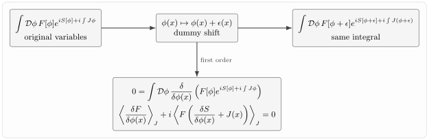
The shift $\phi\mapsto\phi+\epsilon$ leaves the value of the path integral unchanged. Expanding to first order gives an insertion of $\delta S/\delta\phi+J$ and the contact term from differentiating the explicit fields in $F[\phi]$; setting $J=0$ recovers the source-free identity.

For the free scalar action,

$$S_0[\phi]=\int d^4x\,\frac12\left(\partial_\mu\phi\partial^\mu\phi-m^2\phi^2\right),$$

we have

$$\frac{\delta S_0}{\delta\phi(x)}=-(\Box_x+m^2)\phi(x).$$

Choose $F[\phi]=\phi(y)$ and set $J=0$. Since

$$\frac{\delta\phi(y)}{\delta\phi(x)}=\delta^{(4)}(x-y),$$

the Schwinger–Dyson identity gives

$$\delta^{(4)}(x-y)-i(\Box_x+m^2)\langle0|\mathcal T\phi(x)\phi(y)|0\rangle=0.$$

Thus

$$(\Box_x+m^2)G_F(x-y)=-i\delta^{(4)}(x-y),$$

which is precisely the Green-function equation obtained from the explicit momentum-space propagator. The same logic will be used repeatedly: differentiating the action gives equations of motion, while differentiating the insertions gives contact terms.

Operator memory inside a c-number integral

In a path integral the variables $q(t)$ and $\phi(x)$ are ordinary commuting integration variables. This is wonderfully useful, but it can be misleading. The path integral is not saying that quantum operators commute. It is saying that operator information is encoded in the time-ordering prescription, the short-time definition of the measure, and the contact terms generated by differentiating time-ordered products.

The Hamiltonian form of the path integral makes this especially visible:

$$K(q_f,t_f;q_i,t_i) =\int\mathcal Dp\,\mathcal Dq\, \exp\left(i\int_{t_i}^{t_f}dt\,[p\dot q-H(p,q)]\right).$$

The objects $p(t)$ and $q(t)$ inside the integral are c-number histories. Nevertheless, the time-ordered correlator of $p$ and $q$ has the jump required by the canonical commutator. Since

$$[q(t),p(t)]=i,$$

we have

$$[p(t),q(t)]=-i.$$

Thus

$$\boxed{ \lim_{\epsilon\to0^+} \left( \langle\mathcal T p(t+\epsilon)q(t)\rangle - \langle\mathcal T p(t-\epsilon)q(t)\rangle \right) =-i. }$$

This jump is the source of the delta-function term in the oscillator Green function equation. For $p=\dot q$,

$$G_F(t-t')=\langle\mathcal Tq(t)q(t')\rangle$$

has a continuous value at $t=t'$, but its derivative has a discontinuity. Consequently

$$(\partial_t^2+\omega^2)G_F(t-t')=-i\delta(t-t').$$

So the phrase “c-number path integral” should not be read as “classical mechanics.” The integration variables commute, but the limiting prescription knows about quantum commutators.

The paths integrated over in $\int\mathcal Dp\,\mathcal Dq$ are c-number histories, but the time-ordered correlator remembers the operator algebra. Moving $p(t)$ across $q(t')$ produces the jump $[p,q]=-i$, which appears as a delta-function contact term.

A first interacting test

The source formalism is useful because it turns interactions into derivatives. This is the first place where the bookkeeper becomes a calculator: every field in the interaction can be replaced by $(1/i)\delta/\delta J$, acting on the free Gaussian $Z_0[J]$.

Consider an anharmonic oscillator with

$$S[q] =\int dt\left(\frac12\dot q^2-\frac12\omega^2q^2-\frac{\lambda}{4!}q^4\right).$$

The classical equation of motion is

$$(\partial_t^2+\omega^2)q(t)+\frac{\lambda}{3!}q^3(t)=0.$$

The exact two-point function obeys the corresponding quantum equation with a contact term:

$$\boxed{ (\partial_t^2+\omega^2) \langle\mathcal Tq(t)q(t')\rangle +\frac{\lambda}{3!} \langle\mathcal Tq^3(t)q(t')\rangle =-i\delta(t-t'). }$$

This equation is exact, but it is not closed: the two-point function depends on a four-point function. Acting on the four-point function produces a six-point function, and so on. This is the beginning of the Schwinger–Dyson hierarchy.

At first order in $\lambda$, the two-point correction comes from expanding

$$e^{-i\frac{\lambda}{4!}\int dt\,q^4(t)} =1-i\frac{\lambda}{4!}\int dt\,q^4(t)+O(\lambda^2).$$

Expanding the normalized numerator and denominator gives the first-order correction

$$G^{(1)}(t_a,t_b) =-i\frac{\lambda}{4!}\int dt\, \left[ \langle\mathcal Tq(t_a)q(t_b)q^4(t)\rangle_0 -\langle\mathcal Tq(t_a)q(t_b)\rangle_0 \langle q^4(t)\rangle_0 \right].$$

The subtraction removes the three Wick pairings in which the external fields contract with each other and $q^4(t)$ forms a vacuum bubble. The remaining $12$ pairings are connected to the designated interaction vertex: two of the four $q(t)$ factors connect to the external points, and the remaining two contract with each other. This is a statement about diagram topology after the four fields at $t$ are grouped into one vertex, not a nonzero connected six-point cumulant of the free Gaussian theory. Therefore

$$\boxed{ G^{(1)}(t_a,t_b) =-i\frac{\lambda}{2}\int dt\, G_0(t_a-t)G_0(0)G_0(t-t_b). }$$

This is the tadpole correction. It is already visible in ordinary quantum mechanics, and the same combinatorics will reappear in scalar field theory.

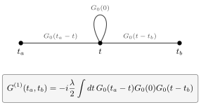
The first connected correction to the two-point function in a $q^4$ interaction is a tadpole insertion. The loop $G_0(0)$ comes from contracting two fields at the same interaction time $t$.

The source functional gives a compact way to generate this expansion. Since

$$\frac{1}{i}\frac{\delta}{\delta J(t)} e^{i\int Jq}=q(t)e^{i\int Jq},$$

a polynomial interaction may be replaced by a polynomial in functional derivatives:

$$Z[J] \propto \exp\left[-i\frac{\lambda}{4!}\int dt\, \left(\frac{1}{i}\frac{\delta}{\delta J(t)}\right)^4\right] Z_0[J].$$

The proportionality reminds us that the final answer must be normalized so that $Z[0]=1$. The next page turns this observation into the systematic perturbative expansion for interacting field theory.

Summary

A source functional packages all time-ordered Green functions into one object. The source $J$ is an auxiliary classical function coupled linearly to the quantum coordinate or field. Functional derivatives with respect to $J$ pull down insertions, and setting $J=0$ returns the physical correlators.

For a free theory, the source functional is Gaussian:

$$Z_0[J]=\exp\left[-\frac12 JG_FJ\right].$$

This equation is the source-functional version of Wick theorem. Two derivatives produce the propagator; higher derivatives produce sums over pairings. The logarithm $\log Z[J]$, or equivalently $W[J]=-i\log Z[J]$, generates connected correlators.

Although the path integral uses c-number histories, it still remembers operator algebra. Contact terms and discontinuities of time-ordered products encode commutators such as $[q,p]=i$. Interactions make the hierarchy of Green functions non-Gaussian, but the source functional remains the natural language: interactions become functional derivative operators acting on $Z_0[J]$.

Common pitfalls

Do not forget the factors of $i$ in source differentiation. With a Lorentzian source coupling $e^{i\int J\phi}$, each field insertion is generated by $(1/i)\delta/\delta J$. Two derivatives of $Z[J]$ therefore carry a minus sign before they become the physical two-point function.

Do not confuse $Z[J]$ with $W[J]$. The functional $Z[J]$ generates full correlators, including disconnected products. The logarithm of $Z[J]$ generates connected correlators.

Do not set $J=0$ before differentiating. The source is a temporary probe; differentiating first and then removing the probe is the whole point of the construction.

Do not confuse normalization with connectedness. Dividing by $Z[0]$ cancels vacuum bubbles, while taking $\log Z[J]$ selects connected diagrams.

Do not treat $Z[0]$ as automatically equal to $1$ unless the normalization has been chosen that way. In perturbation theory, dividing by $Z[0]$ cancels vacuum bubbles.

Do not conclude that c-number path variables commute in the operator sense. The operator commutators are encoded in the time-ordering prescription and the contact terms.

Do not ignore coincident-point factors such as $G_0(0)$. In quantum mechanics they may be finite after a prescription. In field theory they are often ultraviolet divergent and become the first signal of renormalization.

Do not leave the source turned on after differentiation unless the problem explicitly asks for source-dependent in–out data. Ordinary vacuum correlators are obtained by differentiating first and then setting $J=0$. A causal response problem instead requires an in–in or Schwinger–Keldysh prescription.

Exercises

Exercise 1: Differentiating a Gaussian source

Let

$$Z[J]=\exp\left(\frac12J_iA_{ij}J_j\right)$$

where $A_{ij}=A_{ji}$. Compute

$$\left.\frac{\partial^2Z}{\partial J_i\partial J_j}\right|_{J=0}, \qquad \left.\frac{\partial^4Z}{\partial J_i\partial J_j\partial J_k\partial J_\ell}\right|_{J=0}.$$

Solution

The first derivative is

$$\frac{\partial Z}{\partial J_i}=A_{ij}J_jZ.$$

Therefore

$$\left.\frac{\partial^2Z}{\partial J_i\partial J_j}\right|_{J=0}=A_{ij}.$$

For four derivatives, only pairings survive at $J=0$:

$$\left.\frac{\partial^4Z}{\partial J_i\partial J_j\partial J_k\partial J_\ell}\right|_{J=0} =A_{ij}A_{k\ell}+A_{ik}A_{j\ell}+A_{i\ell}A_{jk}.$$

This is the finite-dimensional Wick theorem.

Exercise 2: Lorentzian source signs

For the harmonic oscillator source functional

$$Z_0[J]=\exp\left[-\frac12\int dt\,dt'\,J(t)G_F(t-t')J(t')\right],$$

show that

$$\left.\frac{1}{i^2}\frac{\delta^2Z_0[J]}{\delta J(t_1)\delta J(t_2)}\right|_{J=0} =G_F(t_1-t_2).$$

Solution

Differentiate once:

$$\frac{\delta Z_0}{\delta J(t_1)} =-\left(\int dt'\,G_F(t_1-t')J(t')\right)Z_0[J].$$

Differentiate again and set $J=0$. Terms proportional to $J$ vanish, leaving

$$\left.\frac{\delta^2Z_0}{\delta J(t_1)\delta J(t_2)}\right|_{J=0} =-G_F(t_1-t_2).$$

Since $1/i^2=-1$,

$$\left.\frac{1}{i^2}\frac{\delta^2Z_0}{\delta J(t_1)\delta J(t_2)}\right|_{J=0} =G_F(t_1-t_2).$$

Exercise 3: Connected correlators from the source functional

Use $W[J]=-i\log Z[J]$ to show that the connected two-point function is

$$G_2^{\mathrm{conn}}(x,y) =\left.\frac1i\frac{\delta^2W[J]}{\delta J(x)\delta J(y)}\right|_{J=0}.$$

Then verify this formula for the free scalar field.

Solution

Since $Z=e^{iW}$,

$$\frac{1}{i}\frac{\delta Z}{\delta J(x)} =\frac{\delta W}{\delta J(x)}Z.$$

A second derivative gives

$$\frac{1}{i^2}\frac{\delta^2Z}{\delta J(x)\delta J(y)} =\left(\frac{1}{i}\frac{\delta^2W}{\delta J(x)\delta J(y)} +\frac{\delta W}{\delta J(x)}\frac{\delta W}{\delta J(y)}\right)Z.$$

At $J=0$ and with $Z[0]=1$, this says

$$G_2(x,y)=G_2^{\mathrm{conn}}(x,y)+G_1(x)G_1(y),$$

where

$$G_2^{\mathrm{conn}}(x,y) =\left.\frac1i\frac{\delta^2W[J]}{\delta J(x)\delta J(y)}\right|_{J=0}.$$

For the free scalar field,

$$Z_0[J]=\exp\left[-\frac12\int JG_FJ\right],$$

so

$$W_0[J] =-i\log Z_0[J] =\frac{i}{2}\int JG_FJ.$$

Therefore

$$\left.\frac1i\frac{\delta^2W_0[J]}{\delta J(x)\delta J(y)}\right|_{J=0} =G_F(x-y).$$

Exercise 4: First tadpole correction

For the anharmonic oscillator interaction

$$S_{\mathrm{int}}[q]=-\frac{\lambda}{4!}\int dt\,q^4(t),$$

derive the first-order connected correction

$$G^{(1)}(t_a,t_b) =-i\frac{\lambda}{2}\int dt\, G_0(t_a-t)G_0(0)G_0(t-t_b).$$

Solution

Expand the interaction factor:

$$e^{iS_{\mathrm{int}}} =1-i\frac{\lambda}{4!}\int dt\,q^4(t)+O(\lambda^2).$$

The first-order contribution to the two-point function is

$$G^{(1)}(t_a,t_b) =-i\frac{\lambda}{4!}\int dt\, \left[ \langle\mathcal Tq(t_a)q(t_b)q^4(t)\rangle_0 -\langle\mathcal Tq(t_a)q(t_b)\rangle_0\langle q^4(t)\rangle_0 \right].$$

The subtraction removes the vacuum-disconnected pairings. Every remaining pairing attaches one $q(t)$ to $q(t_a)$, one $q(t)$ to $q(t_b)$, and contracts the two remaining $q(t)$ fields with each other. There are

$$4\cdot3=12$$

ways to choose the two fields connected to the external points. Therefore

$$\langle\mathcal Tq(t_a)q(t_b)q^4(t)\rangle_0 -\langle\mathcal Tq(t_a)q(t_b)\rangle_0\langle q^4(t)\rangle_0 =12G_0(t_a-t)G_0(t-t_b)G_0(0).$$

Multiplying by $-i\lambda/4!$ gives

$$G^{(1)}(t_a,t_b) =-i\frac{\lambda}{2}\int dt\, G_0(t_a-t)G_0(0)G_0(t-t_b).$$

Exercise 5: Contact jump from time ordering

Let

$$G_F(t-t')=\langle\mathcal Tq(t)q(t')\rangle$$

for the harmonic oscillator with $p=\dot q$. Show that the discontinuity

$$\lim_{\epsilon\to0^+}\left[ \partial_tG_F(t-t')\big|_{t=t'+\epsilon} -\partial_tG_F(t-t')\big|_{t=t'-\epsilon} \right] =-i$$

implies

$$(\partial_t^2+\omega^2)G_F(t-t')=-i\delta(t-t').$$

Solution

Away from $t=t'$, the time-ordered two-point function solves the homogeneous oscillator equation:

$$(\partial_t^2+\omega^2)G_F(t-t')=0, \qquad t\ne t'.$$

The only possible distributional contribution is at $t=t'$. If a function is continuous but its first derivative has a jump $A$ at $t=t'$, then its second derivative contains

$$A\delta(t-t').$$

Here

$$A= \partial_tG_F\big|_{t=t'+0} - \partial_tG_F\big|_{t=t'-0} =-i.$$

Therefore

$$(\partial_t^2+\omega^2)G_F(t-t')=-i\delta(t-t').$$

This delta function is the contact term associated with the canonical commutator.

References and further reading

• Mark Srednicki, Quantum Field Theory, Sections 6–9, for the construction of path integrals and generating functionals for free and interacting scalar field theory.
• Sidney Coleman, Lectures of Sidney Coleman on Quantum Field Theory, Chapters 13, 28, and 32, for source functionals, Green functions, and the relation between functional integrals and Feynman rules.
• A. Zee, Quantum Field Theory in a Nutshell, Chapter I.2 and Appendix A, for the path-integral viewpoint and Gaussian source identities.
• Steven Weinberg, The Quantum Theory of Fields, Volume I, Chapter 9 and Appendix A, for path-integral methods, source insertions, and Gaussian multiple integrals.