

Running Couplings and Critical Free Energy
The previous lesson turned the one-loop logarithm in four-dimensional theory into a renormalization-group equation. On the critical trajectory, at a positive infrared scale, the four-point vertex became a running coupling,
and the quadratic operator insertion acquired a running normalization,
These two factors also control critical thermodynamics. Consider the ordinary continuous-transition basin with fixed positive weak quartic coupling and no ordering field. Take the thermodynamic limit first, then approach from the symmetric side with dimensionless reduced temperature , where . In four classical statistical dimensions, the coupling is marginally irrelevant: mean-field powers acquire logarithmic corrections. Equivalently this is a four-dimensional Euclidean field theory; it is not a generic claim about a thermal transition in three spatial dimensions merely because its microscopic quantum theory is relativistic in dimensions.
The main thermodynamic result derived below is the logarithmic singularity of the specific heat in the one-component theory,
up to nonuniversal constants inside the logarithm and in the overall normalization. Equivalently, the singular part of the free-energy density behaves as
at leading-log accuracy. The power follows from two one-loop RG coefficients. The inverse exponential correlation length cuts off the critical running. The asymptotic power requires at fixed positive , as well as controlled weak running; the free-coupling limit cannot be interchanged with this limit. Proportionality leaves the free-energy amplitude and its sign unspecified: the physical heat capacity is .
Sliding the cutoff
Section titled “Sliding the cutoff”Quartic and thermal running
Section titled “Quartic and thermal running”Use the critical leading-log flow at positive scales , in the normalization
For one real scalar field,
where appears in the four-point coupling and appears in the insertion:
It is often cleaner to use
so that
Within this leading local approximation, the running coupling describes the four-point vertex at scale with fixed microscopic cutoff . The same flow composes changes of cutoff while preserving the retained low-energy vertex. Finite matching terms and higher-derivative operators lie beyond this formula; a fixed massive theory also leaves the critical running regime below its mass scale.
Indeed,
Suppose we lower the cutoff from to , with . To leave the leading-log vertex at unchanged, the new bare coupling must satisfy
Therefore
The modes between and contribute to the new quartic coefficient. The figure shows this composition of the retained flow, rather than an exact equality of the full cutoff actions.
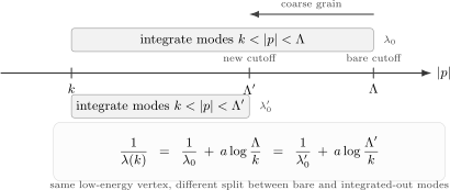
For , the same leading-log vertex follows from either cutoff and its matched quartic coefficient. The diagram suppresses finite matching terms and the other operators of the full effective action.
There is a sign convention hiding here, and it is worth making it explicit. If is the probe momentum, then
For positive , raising the probe scale increases the coupling, while lowering the probe scale decreases it. If instead we use the logarithmic coarse-graining variable
then
These are the same statement. The sign changes because increasing means moving toward the infrared.
Landau–Ginzburg theory as Euclidean field theory
Section titled “Landau–Ginzburg theory as Euclidean field theory”To apply this to critical phenomena, consider a one-component order parameter , such as the coarse-grained magnetization of an Ising-like ferromagnet. Near a continuous transition, the Landau–Ginzburg functional has the local form
The classical statistical partition function is
In practice one absorbs the factor into the parameters of the functional. The mathematical object is then a Euclidean scalar field theory. The mass parameter is the thermal tuning parameter:
The subtraction by is essential. Ultraviolet fluctuations shift the critical temperature. The physical transition is not located by the naive condition , but by the condition that the inverse correlation length vanish.
The order-parameter two-point function diagnoses a particular spectral channel. In the symmetric phase , so it is already connected. In a transfer-matrix setting, treating the separation direction as Euclidean time and writing a sum over its spectral states gives
The decay rate is the lowest positive spectral support with nonzero overlap, not necessarily the first excited level of the entire theory. In infinite volume the sum can become an integral; a continuum threshold may add a power prefactor to the exponential. The spectral representation makes this channel restriction explicit. At this transition the order-parameter decay scale vanishes and the exponential correlation length
becomes large. We use this scale to stop the leading-log flow. A mass defined by a zero-momentum subtraction or a second moment need not equal exactly; their identification requires the corresponding single-pole or retained perturbative approximation, as discussed in mass tuning.
The upper critical dimension of theory is . The quartic coupling has zero engineering dimension, but at fixed positive and it becomes irrelevant logarithmically:
This slow drift to zero is why mean-field powers survive but logarithms do not disappear.
Reduced temperature and the flow-stopping scale
Section titled “Reduced temperature and the flow-stopping scale”Let
be the reduced temperature already used above. On the symmetric side , the leading mean-field identification of the decay scale is
so, with fixed dimensionful proportionality factors understood, the critical RG flow stops at
In four dimensions, the relation between and itself receives logarithmic corrections because the thermal scaling field runs. For the leading powers of large logarithms derived in this page, this distinction only changes subleading terms inside
Indeed, replacing gives
and the leading power becomes the same leading power of . Constants inside a dimensionless logarithm affect only subleading terms; a dimensional temperature difference cannot itself be its argument.
The thermal operator
Section titled “The thermal operator”The leading singular specific heat comes from two derivatives with respect to the thermal scaling coordinate, whose temperature derivative is assumed finite and nonzero at . Other parameter dependences contribute analytic backgrounds or subleading terms in this critical basin. The operator conjugate to the local quadratic coefficient is
This is the thermal operator. After separating analytic backgrounds and local source-contact terms, the leading singular temperature response is, up to nonuniversal constants,
where the connected correlator is understood. Local products and their contact terms require the same composite-source prescription. In momentum space, define
The thermodynamic response uses , whereas the massless critical correlator at nonzero Euclidean momentum uses as an infrared probe. The mass cuts off the thermodynamic response. Setting matches their leading infrared logarithms, not their complete finite values.
The thermal operator is the quadratic insertion from II06. Its dimensionless two-leg factor is defined by the local shell flow at positive RG scale , with the remaining infrared modes excluded. It is not the full massless zero-transfer insertion vertex: nonzero scalar-leg momentum alone does not regulate that vertex’s insertion loop. The local RG equation
has the solution
The factor should not be confused with a new coupling. It is a normalization factor for a local operator insertion. Depending on convention, one may say that the source runs, or that the operator runs, or that the vertex associated with the insertion runs. Correlation functions only depend on the combined normalization.
Specific heat from two thermal insertions
Section titled “Specific heat from two thermal insertions”The leading contribution to is the bubble with two insertions. In the free massless theory in four dimensions, at ,
The interacting leading-log result is obtained by slicing this logarithmic integral into shells. Each shell at scale sees two dressed thermal insertions, so
where is a positive constant depending on the normalization of . Here denotes the shell-accumulated response, with its ultraviolet matching value at , not the thermodynamic correlator at zero momentum. The logarithmic exponent is universal within this critical class; the overall coefficient is not.
This formula is intentionally differential in . A single shell contributes the free-theory logarithmic measure, while the accumulated effect of harder shells is already contained in the two factors of . This avoids double-counting the same logarithms.
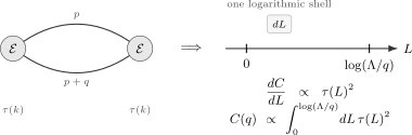
The singular specific heat is the integrated connected two-point function of the thermal operator . At leading-log accuracy, a logarithmic shell contributes an amount proportional to .
Using
we find
The integral is elementary:
Thus, at fixed positive and ,
at leading-log accuracy. The exponent is positive even though each individual insertion factor decreases. The reason is simple: the heat capacity integrates over all logarithmic shells. The integrand decreases as , but the accumulated integral still grows as .
Away from the critical point, the RG stops when reaches the physical mass
Therefore
To leading mean-field accuracy,
so fixed reference scales change subleading terms while the factor of is absorbed into the overall amplitude, and
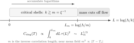
On the symmetric side , the inverse exponential correlation length cuts off the critical running. Matching the logarithmic shells at gives the leading singular heat capacity; it does not equate the full massive response with the critical momentum-dependent correlator.
The singular free-energy density follows by integrating twice with respect to the thermal scaling variable. Since the mean-field specific-heat exponent is , its leading power is , where is a mass-squared scaling coordinate proportional to near the transition. Introduce a fixed positive reference of the same dimension. The logarithm is inherited from :
up to subleading logarithms and nonuniversal amplitudes, including the sign required by . The Gaussian fixed point controls the leading powers while the marginally irrelevant coupling controls the logarithmic correction. The thermal flow and background-subtracted heat-capacity equation are developed in Zinn-Justin 2021, § 17.2, pp. 423–425.
Why four dimensions is special
Section titled “Why four dimensions is special”The logarithm in the heat capacity is already visible in the free bubble integral
For and nonzero Euclidean momentum, the integral without a UV cutoff is convergent: both soft regions are integrable and the large-momentum tail converges. Rescaling by gives its leading nonlocal part for ,
while is the logarithmic ultraviolet boundary of this range. In the region ,
Thus is the dimension in which every decade of momenta contributes comparably. That is exactly when the RG is needed to sum a long chain of logarithmic shells.
For , the quartic coupling has negative engineering dimension:
It is irrelevant already by power counting. Loop corrections shift local parameters, including the critical temperature, but they do not generate the same universal logarithmic scaling. In five dimensions, for example,
is dominated by cutoff-dependent local terms. These terms must be absorbed into the location of the critical point and other nonuniversal coefficients.
For with small positive , the quartic coupling is relevant at the Gaussian fixed point and the Wilson–Fisher fixed point is perturbatively controlled. In its critical basin, non-mean-field powers replace the four-dimensional logarithms. Extending that statement to other dimensions requires the appropriate universality-class evidence; see critical exponents and the limits of hyperscaling.
O(N) aside
Section titled “O(N) aside”For fixed positive integer in the symmetric-side critical basin, with the same local leading-log prescription, the one-loop coefficients become
where is the coefficient for the thermal operator . Hence
The specific heat receives two thermal insertions. Using the large- tail only above a fixed positive matching scale where gives
For , this gives the divergent logarithmic singularity
The Ising case gives . The case is marginal inside the logarithmic correction itself and gives a further logarithm, , at this level of approximation. For , the shell integral converges as : the heat capacity approaches a nonuniversal constant, with a leading nonanalytic correction whose magnitude scales as . Thus a negative power here describes a finite cusp correction, not a heat capacity that literally vanishes.
Summary
Section titled “Summary”Within the retained leading-log approximation, changing the cutoff from to is compensated by changing the quartic coefficient so that
The retained vertex at scales well below both cutoffs is unchanged; finite matching terms and other effective operators are not specified by this identity.
The Landau–Ginzburg theory of a scalar order parameter is a Euclidean field theory. Its quadratic coefficient is the thermal tuning parameter,
and the thermal operator is
At the four-dimensional upper critical dimension, the quartic coupling is marginally irrelevant:
The local thermal insertion at positive shell scale has the leading-log normalization
After separating analytic and contact backgrounds, the singular specific heat is the integrated connected thermal correlator. For fixed positive and , the shell contributions give
Using at leading mean-field order gives
up to subleading changes inside the large logarithm. Integrating twice with respect to temperature gives
Common pitfalls
Section titled “Common pitfalls”A logarithm needs a dimensionless argument. On the stated symmetric-side approach, use the positive large quantity , or the corresponding ; neither the dimensional difference nor can appear alone inside a logarithm.
Do not set the critical point by the bare condition . Fluctuations shift the critical temperature. The correct tuning is , where the physical mass vanishes.
Do not conclude that because in the infrared, the result is exactly Gaussian. The approach to the Gaussian fixed point is logarithmically slow, and operator insertions accumulate anomalous logarithmic factors.
Do not identify with the full thermodynamic response . Their leading logarithms match at , while their finite terms and infrared completion differ.
Do not treat cutoff-dependent constants in the free energy as universal. The location of , additive constants in , and analytic background terms depend on microscopic physics. The logarithmic singularity is the universal object.
Exercises
Section titled “Exercises”Exercise 1 — Cutoff redefinition invariance
Section titled “Exercise 1 — Cutoff redefinition invariance”Within the retained leading-log ansatz, take and positive . Show explicitly that the running coupling
is invariant under the replacement if is replaced by
Solution
With the new cutoff and new bare coupling, the low-energy coupling is
Substitute the proposed relation:
The logarithms combine:
Therefore
so .
Exercise 2 — Running of the thermal insertion
Section titled “Exercise 2 — Running of the thermal insertion”Use positive and the local insertion at positive RG scale, with finite . Let
Solve for , and evaluate the exponent for
Solution
Divide by :
Integrating from to gives
The integral is
Therefore
For the one-component theory,
so
Exercise 3 — The specific-heat logarithm
Section titled “Exercise 3 — The specific-heat logarithm”For positive and finite , assume the shell-accumulated heat-capacity response obeys
Show that when at fixed positive .
Solution
Integrate:
Set
Then
Since
we get
For large ,
up to a nonuniversal multiplicative constant.
Exercise 4 — The four-dimensional massless bubble
Section titled “Exercise 4 — The four-dimensional massless bubble”For nonzero Euclidean momentum with , use Feynman parameters to show that the massless four-dimensional bubble
has a logarithmic dependence on . Work only to this accuracy: replacing the shifted sharp-cutoff domain by a centered one changes nonlogarithmic terms and is not an exact regulated identity.
Solution
Use
With and , shift
Then
Thus
up to cutoff-shape effects that only change nonlogarithmic terms. The standard logarithmic integral gives
Therefore
The -dependent part contributes only a constant, so
The precise additive constant depends on the regulator, but the logarithmic dependence does not.
Exercise 5 — The O(N) logarithmic exponent
Section titled “Exercise 5 — The O(N) logarithmic exponent”For fixed positive integer in the same symmetric-side critical regime, take
Assuming
in the tail at fixed positive , determine the leading heat-capacity behavior for , , and . The lower-scale contribution is a finite matching background. For , show that the divergent part is
Solution
The thermal correlator has two thermal insertions, so
At large ,
The ratio of coefficients is
Therefore
For , an antiderivative has the power
The exponent is
Thus, for ,
When , the exponent of the integrand is , so the integral gives a logarithm of a logarithm:
For , the large- integrand is integrable. The full heat capacity approaches a cutoff-dependent constant , while the leading critical correction obeys
The negative exponent makes this correction vanish at criticality; it describes a finite cusp rather than a divergence.
References
Section titled “References”- Zinn-Justin, Jean. Quantum Field Theory and Critical Phenomena. 5th ed. Oxford University Press, 2021. DOI: 10.1093/oso/9780198834625.001.0001.
Further reading
Section titled “Further reading”- Schwartz, Matthew D. Quantum Field Theory and the Standard Model. Cambridge University Press, 2014, chapter 23.
- Srednicki, Mark. Quantum Field Theory. Cambridge University Press, 2007, sections 28–29.
- Weinberg, Steven. The Quantum Theory of Fields, Volume II: Modern Applications. Cambridge University Press, 1996, sections 18.2, 18.5, and 18.8.
- Wilson, Kenneth G., and Michael E. Fisher. “Critical Exponents in 3.99 Dimensions.” Physical Review Letters 28 (1972): 240–243.