

Random Lattices, Matrix Models, and Random Surfaces
A Hermitian matrix integral generates oriented polygonal surfaces because its index contractions retain the cyclic order around every vertex. The power of the matrix size counts genus; a critical coupling controls the large-area tail. We will derive both statements for the quartic one-matrix model, keeping its formal positive-weight map expansion distinct from a convergent matrix integral.
The geometric starting point is the distinction between coordinates and intrinsic distance in the preceding lesson. The later matter discussion uses the Euclidean Polyakov action and the zero-mode and Liouville qualifications.
Random polygonal geometry
Section titled “Random polygonal geometry”A regulator for fluctuating geometry need not randomize connectivity: one can also vary lengths or metric data on fixed combinatorics. Here we choose a specific alternative, a sum over connected closed oriented polygonal maps. Assigning an equilateral metric to each polygon turns the combinatorial gluing into a piecewise-flat intrinsic geometry. No embedding in a background plane is required.
Let be the number of faces and their common physical area. At a fixed topology, a schematic sum is
Here has units of inverse area, and the automorphisms preserve the orientation and polygonal incidence data. The dimensionless face fugacity is , possibly with a microscopic normalization absorbed into it. A finite map has finitely many field variables; convergence still requires a suitable action and treatment of zero modes.
Graph distance counts links. Multiplying it by their length gives a path metric restricted to edges, which need not equal the unrestricted piecewise-flat geodesic distance. Curvature, in contrast, has an immediate local description. For equilateral triangles, if triangles meet at ,
The last identity is for a closed oriented surface of genus . Indeed, and turn the sum of deficit angles into .
Matrix contractions and closed ribbon surfaces
Section titled “Matrix contractions and closed ribbon surfaces”An ordinary scalar Wick contraction pairs individual lines. A matrix contraction pairs two indices and therefore supplies the extra information needed to construct a surface. Take a dimensionless Hermitian matrix with
For real this integral converges on Hermitian matrices; is Gaussian. For real the potential is unbounded below. In that region we use its formal Wick expansion, whose coefficients count maps positively. Continuation of those coefficients or of a specified saddle branch does not select a unique integration contour or nonperturbative completion.
Gaussian normalization gives
The two Kronecker deltas make an edge a ribbon; the trace gives the cyclic order at a vertex. Replace each vertex by an oriented disk and join its incident ribbons in that order. This thickening has a boundary. Each closed index loop is one boundary component. Cap every boundary component with a disk to obtain the closed oriented surface whose genus we count. This construction is the geometric content of the matrix expansion in Di Francesco, Ginsparg and Zinn-Justin 1994, §1.2, printed preprint pp. 7–10, PDF.
The resulting objects are cellular maps. Loops, multiple edges and polygonal self-identifications are allowed; the integral does not restrict itself to simple square meshes. In the dual map each quartic vertex becomes a quadrilateral face. Thus interaction vertices count dual faces.
The large-N genus expansion
Section titled “The large-N genus expansion”For a connected vacuum graph with vertices, ribbons and index loops, the factors of and are
The remaining numerical symmetry factor is fixed by the expansion of the exponential and the vertex factor . The logarithm selects connected graphs; the Gaussian denominator removes the empty vacuum. Consequently,
At fixed coupling, handles cost . This is the same topology bookkeeping as a closed-string expansion with bare .
The three pairings of one quartic vertex
Section titled “The three pairings of one quartic vertex”Label the four successive matrix factors by , and let be their cyclic order. A Wick pairing is a fixed-point-free involution . Following a ribbon and then the next vertex side gives the face permutation , with applied first.
| Pairing | Cycles of | Capping disks | Genus |
|---|---|---|---|
| 3 | 0 | ||
| 3 | 0 | ||
| 1 | 1 |
All three have and . Each contributes to the Gaussian trace moment. Hence
This fixes the normalization of the planar and torus generating functions, not just their powers of . The diagram compares one of the two planar pairings with the one-handle pairing; inspect the boundary cycles before capping them.
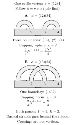
For and , the pairing has three boundary cycles, while has one. Thickening the vertex and ribbons, then capping each boundary with a disk, gives : a sphere or a torus. The other planar pairing, , is not redrawn. At the lower projected crossing, dashed pieces continue the same strands behind the other ribbon; the crossing adds no vertex, twist or gluing. These are schematic contractions in the formal quartic counting model; each labeled planar pairing contributes , and the genus-one pairing contributes .
The normalized quartic eigenvalue density
Section titled “The normalized quartic eigenvalue density”Diagonalize . The Jacobian is the square of the Vandermonde determinant,
After the angular integral, the partition function is proportional to
The omitted factor is independent of and cancels in . Differentiating the exponent and taking the large- limit gives
On the real stable branch this is an equilibrium density. We continue the solution connected to the Gaussian point into the positive formal counting branch. Introduce
For one symmetric cut , the jump condition and polynomial potential suggest
where at infinity. The coefficient of cancels by construction. Requiring the coefficient of to be one fixes
We choose at , so there. Taking the discontinuity yields the normalized density
Outside this interval the density is zero. At it reduces to . For its polynomial prefactor is smallest at the endpoints, where its value is . At
the endpoint zero changes from a square root to a three-halves power. The critical density still integrates to one. It is a solution on the formal counting branch, not a probability measure defined by the divergent positive- matrix integral.
For comparison, Di Francesco, Ginsparg and Zinn-Justin 1994, §2.1, printed preprint pp. 15–19, Eqs. (2.3)–(2.27), PDF use an exponent . Starting at , set and . Their resolvent has denominator , so ours is . Their becomes our . The Jacobian must also be retained when comparing unnormalized partition functions.
Critical area counting
Section titled “Critical area counting”The planar generating function counts unmarked spherical maps with the symmetry weights fixed above:
Its derivative is a density moment,
The middle equality follows by integrating powers against , for example with . At it gives , in agreement with the two planar Wick pairings.
Put . Expanding at the critical point gives
The second expression is the leading nonanalytic term, obtained using ; analytic background terms remain in the full function. Thus , and stay finite at , while diverges.
The generalized binomial formula gives
For noninteger , the large- ratio of the Gamma functions therefore converts the singularity into
Equivalently, with the pure-gravity string susceptibility . The coefficient here is specific to our action and unmarked-map normalization. The fixed-area interpretation and susceptibility convention are developed in Di Francesco, Ginsparg and Zinn-Justin 1994, §1.3, printed preprint pp. 11–12, PDF.
A divergent mean is not a fixed-area limit
Section titled “A divergent mean is not a fixed-area limit”At , the unmarked weights decay as : both their sum and their first area moment converge. Two ordered face marks, with coincidence allowed, instead multiply each coefficient by :
For , this defines a positive normalized area distribution. Its mean is
The partition sum approaches , but the mean diverges. This does not imply that a sample has finite nonzero area when its face area tends to zero. The critical marked weights have tail . For any fixed , uniformly as ,
Here the normalization is bounded below for in a fixed interval just below . Rare large maps can make the mean diverge even as physical area tends to zero in probability.
A fixed-area scaling limit instead conditions on and takes with prescribed. This specifies area scaling. Convergence of random metric spaces, and the appropriate rescaling of graph distances, require their own results; they do not follow from alone. In fugacity language the critical shift can be written , so .
Double scaling and the torus logarithm
Section titled “Double scaling and the torus logarithm”At fixed , large selects the sphere. Tuning to changes the relative weights of genera. For this pure-gravity branch the leading singular terms have the form
Genus one is logarithmic, not a nonsingular zeroth power. One can check its coefficient from the even-potential double-scaling equations in Di Francesco, Ginsparg and Zinn-Justin 1994, §2.5, printed preprint pp. 29–32, Eqs. (2.66)–(2.68), PDF. In their scaled variables the logarithm and specific heat satisfy
Substituting gives . Therefore
up to integration terms. Since is proportional to , the coupling-dependent logarithm is ; the accompanying and constant scale terms are separated with the background subtraction. The coefficient is tied to this even quartic normalization.
The combined limit keeps
fixed. For , then becomes a power of , retaining every genus after analytic backgrounds are subtracted. This effective critical coupling differs from the bare topology parameter .
The construction determines a formal continuum genus expansion. It does not choose a unique nonperturbative theory: different completions can share this expansion while differing exponentially, as explained in Di Francesco, Ginsparg and Zinn-Justin 1994, §7.2, printed preprint pp. 97–98, PDF. Likewise, factorial growth when all topologies are allowed is compatible with the finite-radius planar series derived above.
Matter, zero modes, and the conformal factor
Section titled “Matter, zero modes, and the conformal factor”To add matter, use a connected finite triangulated surface and target coordinates with positive Euclidean norm. A discrete Dirichlet action is
Choose weights for which the quadratic form is positive on nonconstant fields. Equilateral weights or the assembled finite-element Dirichlet form provide examples; individual cotangent weights need not all be positive. With length-valued , has units of inverse length squared and the weights are dimensionless.
Every difference is unchanged by , so the unrestricted Gaussian integral contains an infinite target-translation volume. A definite finite-map convention is to pin one vertex, , and define
The reduced graph quadratic form is positive definite. This pinning convention must be included in the map weights. It is not identical to silently dropping the zero eigenvalue: with the flat vertex measure and vertices, the normalized constant coordinate is times the common translation . Dividing the original integral by instead leaves a factor multiplying the orthogonal nonzero-mode integral.
On a fixed smooth geometry and suitable refining meshes, the local energy approaches
In two dimensions each squared edge difference contributes order , while the number of edges per fixed area is order . There is no extra multiplying the discrete action. This consistency argument does not establish convergence of the random-map sum or its quantum measure.
Two different continuum settings must now be distinguished. For two-dimensional gravity with an area coupling, a formal expression is
with topology, zero-mode normalization and regulator specified. Under the matter action is classically invariant, but
Thus the nonzero area coupling is not an action on a quotient. Writing leaves a physical conformal factor, with the quantum anomaly and a renormalized area operator described by Liouville theory in the previous lesson.
In the distinct critical bosonic string setting, with no such worldsheet area term, Weyl transformations can be gauge redundancies only if the full measure is anomaly-free. The free embedding scalars contribute and reparametrization ghosts contribute , giving the familiar necessary local cancellation . That test neither removes the displayed classical area variation nor proves existence of the path integral. General matter changes the susceptibility, and arbitrary is not automatically in the real spacelike Liouville regime of the earlier lesson.
Integrated vertex operators
Section titled “Integrated vertex operators”Classically, a surface embedded in target space has a target-space density and its Fourier transform,
Integrating with the invariant measure makes these expressions reparametrization-invariant. Quantum products at one point must be renormalized. For free bosons with the action above, use the normal-ordered operator . After dividing out the constant target volume, a neutral two-point function on the flat worldsheet obeys
The exponent follows from and the Gaussian contraction identity; fixes the subtraction scale. Nonneutral insertions need a corresponding zero-mode or state prescription.
Here is the positive Euclidean target norm. In a Weyl-gauged string amplitude the local renormalized integrand must have weights , possibly with oscillator factors or dressing; integration alone does not supply that condition. For the exponential alone it requires before any Lorentzian continuation. In two-dimensional gravity the area insertion and the matter operator instead require their appropriate gravitational dressing. These are different uses of reparametrization-invariant expressions.
A further classical example is
It resolves the local tangent contribution in target space. Its quantum definition also requires a composite-operator prescription; the classical coordinate-invariance argument does not settle operator mixing.
Common pitfalls
Section titled “Common pitfalls”Capping is part of genus counting. A thickened ribbon graph has boundary. The index faces become disks of a closed surface only after those boundary components are capped.
Positive counting is formal here. A nonnegative planar density does not repair the divergent positive-coupling real quartic integral.
Topology, area, and distance have different limits. Large suppresses handles. Critical fugacity controls area singularities. A divergent marked mean neither fixes a typical physical area nor establishes a metric scaling limit.
An area term is not Weyl-invariant. Reparametrization invariance, quantum anomaly cancellation, and gravitational dressing address distinct conditions.
The Library separates two tools combined in this lesson: Double-Line Counting and the Topological Expansion explains the powers of matrix size assigned to ribbon graphs, while Matrix Eigenvalue Saddles, Loop Equations, and Phase Transitions develops the resolvent and eigenvalue-density method. Their limiting assumptions help distinguish a formal map expansion from a stable matrix integral.
Exercises
Section titled “Exercises”Genus weight of a ribbon graph
Section titled “Genus weight of a ribbon graph”Consider the Hermitian matrix model with Gaussian propagator
and quartic interaction . Show that a connected ribbon vacuum graph with vertices, propagators, and index faces carries the factor
Then interpret this power in terms of the genus of the corresponding surface.
Solution
Each quartic vertex comes from the interaction term and contributes a factor proportional to . Therefore vertices contribute
Each propagator contributes a factor , so propagators contribute
Every closed index loop is freely summed from to , so every face contributes a factor . Hence faces contribute
Multiplying the factors gives
For a connected orientable ribbon graph, thickening gives a surface with boundary. Capping each of its index-boundary components with a disk gives a closed orientable surface with Euler characteristic
Thus the graph carries the topological weight
Planar diagrams have and scale as . A one-handle correction has and scales as .
Eigenvalue saddle equation
Section titled “Eigenvalue saddle equation”Diagonalize a Hermitian matrix , with . Assuming the measure contains the Vandermonde factor , derive the large- saddle equation
Solution
The eigenvalue representation of the matrix integral is
The exponent is
The saddle equation for is
Thus
At large , define
The sum becomes a principal-value integral because the term is omitted:
This gives
Critical coefficients and singular behavior
Section titled “Critical coefficients and singular behavior”Suppose is noninteger and the unmarked planar map coefficients behave as
Show that the singular part of
has the form
up to analytic terms and a nonuniversal constant.
Solution
Near , define
The large- tail controls the nonanalytic part. Its model sum is a polylogarithm:
After subtracting analytic terms of order lower than the leading nonanalytic term (none if ), the small- expansion contains
The same result follows by replacing only the large- tail by a Laplace integral and treating its lower endpoint by analytic subtraction. Therefore
Since is proportional to near criticality,
For noninteger this is the nonanalytic critical behavior. At nonnegative integer exponents the continuation instead produces logarithms; negative integer exponents give poles. Analytic terms depend on small and are not fixed by the coefficient asymptotics.
Reparametrization invariance of an integrated vertex
Section titled “Reparametrization invariance of an integrated vertex”Show that the integrated vertex operator
is invariant under worldsheet reparametrizations, assuming is a scalar field on the worldsheet.
Solution
Under a reparametrization , the scalar field satisfies
The area element transforms as a density:
Therefore
So is reparametrization-invariant. This does not yet guarantee Weyl invariance. For a physical string vertex operator, the integrand must also have the correct conformal weight.
Continuum limit of the lattice Dirichlet action
Section titled “Continuum limit of the lattice Dirichlet action”Take a quasi-uniform, shape-regular, nondegenerate sequence of triangulations refining a fixed smooth surface, and vertex samples of a smooth, slowly varying field . Use finite-element weights with continuum normalization . For one such triangulation , consider
Explain why this is the natural discrete analogue of
Solution
On a fine triangulation, neighboring vertices are separated by a proper distance of order the lattice spacing. If varies slowly across the lattice, then along an edge
where is the edge scale and is a unit tangent direction on the triangulation. Each squared difference is therefore of order . A two-dimensional region of fixed area contains order edges, so these powers cancel. Under the stated fixed-geometry refinement assumptions, the finite-element sum approaches the Dirichlet energy:
The weight convention fixes , so the matching is . Exact finite-element normalization sets . An additional factor would double-count the derivative scaling in two worldsheet dimensions. This local consistency statement does not prove convergence of an ensemble of random metrics.
References
Section titled “References”- Di Francesco, P., Ginsparg, P., and Zinn-Justin, J. “2D Gravity and Random Matrices.” Physics Reports 254 (1995): 1–133. DOI. Open PDF: arXiv hep-th/9306153v2, 27 July 1994. Locators above use the printed preprint pagination.