Sigma-Model Instantons and Topological Charge

The previous page explained why a continuous order parameter is fragile in two dimensions. The $O(3)$ nonlinear sigma model has no ordinary long-range Néel order in infinite two-dimensional Euclidean spacetime. But the model still has something rigid: topology. Localized configurations with a fixed value at infinity are maps from a compactified spacetime sphere to a target sphere, and such maps fall into disconnected integer-labeled sectors.

Those sectors are invisible in perturbation theory around a constant field. A small fluctuation cannot change how many times the spacetime sphere wraps the target sphere. The nontrivial sectors are represented by finite-action Euclidean saddle points called instantons. In the $O(3)$ model they are especially beautiful: the action satisfies a topological lower bound,

$$S_0\ge {4\pi\over \alpha_0}|Q|,$$

and the configurations that saturate the bound are holomorphic maps between two Riemann spheres. This page builds that statement from scratch.

Required background. Nonlinear sigma models and constraints supplies the $O(3)$ action and target-space geometry.

Helpful background. Spin chains and theta terms motivates the theta angle, while symmetry restoration explains why topology remains informative even without a local order parameter.

Localized fields compactify the plane

Normalization for this page. We work in two Euclidean dimensions with coordinates $x^1,x^2$ and

$$\epsilon_{12}=+1, \qquad z=x^1+ix^2, \qquad \partial_z={1\over2}(\partial_1-i\partial_2), \qquad \partial_{\bar z}={1\over2}(\partial_1+i\partial_2).$$

The $O(3)$ nonlinear sigma model is

$$S_0[\mathbf n] ={1\over2\alpha_0}\int d^2x\,\partial_\mu\mathbf n\cdot\partial_\mu\mathbf n, \qquad \mathbf n^2=1.$$

The topological charge is

$$Q[\mathbf n] ={1\over8\pi}\int d^2x\,\epsilon_{\mu\nu}\, \mathbf n\cdot(\partial_\mu\mathbf n\times\partial_\nu\mathbf n).$$

With these signs, holomorphic $w(z)$ configurations below have $Q>0$ and action $S_0=4\pi Q/\alpha_0$.

A localized instanton has finite Euclidean action, so its gradients die sufficiently fast at infinity:

$$\int_{|x|\gg1} d^2x\,(\partial_\mu\mathbf n)^2<\infty.$$

For the sector decomposition on the plane, we also impose the standard vacuum boundary condition

$$\mathbf n(x)\longrightarrow \mathbf n_\infty \qquad \text{as } |x|\to\infty.$$

The distinction matters: finite Dirichlet energy by itself need not force an arbitrary off-shell field to have a unique pointwise limit at infinity. The compactification argument applies to the localized configuration space with the boundary condition above, which includes the smooth instanton saddles studied here.

The point at infinity can therefore be added to the Euclidean plane. Topologically,

$$\mathbb R^2\cup\{\infty\}\simeq S^2.$$

Since the target space is also $S^2$, a localized field with this boundary condition is a map

$$\mathbf n:S^2_{\rm spacetime}\longrightarrow S^2_{\rm target}.$$

Such maps are classified by the homotopy group

$$\pi_2(S^2)=\mathbb Z.$$

The integer is the degree of the map: how many times the domain sphere covers the target sphere, counted with orientation.

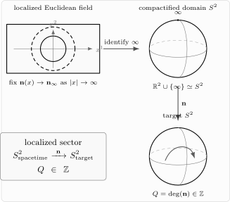
The localized boundary condition makes every direction at Euclidean infinity approach one target point. Thus the plane compactifies to $S^2$, and the field becomes a map $S^2\to S^2$ with integer degree $Q$.

This is already a major difference from ordinary perturbation theory. Around the trivial vacuum, one writes

$$\mathbf n=(\sqrt{1-\boldsymbol\pi^2},\boldsymbol\pi),$$

and expands in small $\boldsymbol\pi$. Such fields live inside one coordinate patch of the target sphere and have $Q=0$. No finite-order perturbative diagram can see a configuration that wraps the entire target.

Circle maps as a warm-up

The same global idea is easiest to see one dimension lower. Let $t\in[0,1]$ parametrize a circle by identifying its endpoints, and consider a map to a target circle,

$$U(t)=e^{i\varphi(t)}.$$

Continuity of $U$ requires only

$$\varphi(1)-\varphi(0)=2\pi k, \qquad k\in\mathbb Z,$$

because $\varphi$ is an angular coordinate. Its winding number is

$$k={1\over2\pi}\int_0^1dt\,{d\varphi\over dt}.$$

The integrand is locally a derivative, yet the integral need not vanish because $\varphi$ need not be a single-valued real function on the circle. The $S^2\to S^2$ charge below is the two-dimensional version of this distinction between a local coordinate formula and global topology.

Topological charge as pulled-back area

The formula for $Q$ becomes transparent in target spherical coordinates. Write

$$\mathbf n=(\sin\Theta\cos\Phi,\sin\Theta\sin\Phi,\cos\Theta).$$

A short calculation gives

$$\mathbf n\cdot(\partial_\mu\mathbf n\times\partial_\nu\mathbf n) =\sin\Theta\,(\partial_\mu\Theta\,\partial_\nu\Phi-\partial_\nu\Theta\,\partial_\mu\Phi).$$

Therefore

$$Q ={1\over4\pi}\int d^2x\, \sin\Theta\,(\partial_1\Theta\,\partial_2\Phi-\partial_2\Theta\,\partial_1\Phi).$$

Equivalently,

$$Q={1\over4\pi}\int \sin\Theta\,d\Theta\wedge d\Phi.$$

The two-form

$$\omega={1\over4\pi}\sin\Theta\,d\Theta\wedge d\Phi$$

is the normalized area form on the target sphere:

$$\int_{S^2}\omega=1.$$

The expression for $Q$ is the integral of the pullback of this area form to the domain sphere. A map that covers the target once with positive orientation has $Q=1$; one that covers it once with reversed orientation has $Q=-1$; a map covering it $k$ times has $Q=k$.

As a check, take the identity map from the domain sphere with angles $(\vartheta,\varphi)$ to the target sphere,

$$\Theta=\vartheta, \qquad \Phi=\varphi.$$

Then

$$Q={1\over4\pi}\int_0^\pi d\vartheta\int_0^{2\pi}d\varphi\,\sin\vartheta=1.$$

The integral is integer-valued for smooth localized configurations with the stated boundary condition, but the density is not itself quantized. The topological charge is global: it knows how local oriented area elements fit together over the whole sphere.

A useful mental check is that $Q$ is stable under smooth deformations that preserve the boundary condition, but not under arbitrary singular ones. To change $Q$, the field must become singular, change its value at infinity, or leave the target sphere. This is why perturbation theory around a smooth vacuum cannot move between sectors.

The closed-domain hypothesis

The integer classification here uses the compactified plane, equivalently a closed domain sphere. On a region with a physical boundary, the bulk integral need not be an integer until boundary data are specified. A constant boundary map can be capped by a disk to recover the closed-sphere degree; a nonconstant boundary map requires its own boundary analysis and can make a theta term affect boundary dynamics.

The theta term is locally a total derivative

The topological density may be written locally as a total derivative. In the spherical patch that excludes the south pole,

$$q(x) ={1\over4\pi}\epsilon_{\mu\nu}\sin\Theta\,\partial_\mu\Theta\,\partial_\nu\Phi ={1\over4\pi}\epsilon_{\mu\nu}\partial_\mu\left[(1-\cos\Theta)\partial_\nu\Phi\right],$$

where

$$Q=\int d^2x\,q(x).$$

This formula explains why the theta term does not change the local classical equation of motion. The Euclidean path integral with theta angle is organized as

$$Z(\theta)=\sum_{Q\in\mathbb Z} e^{i\theta Q}\int_{Q}\mathcal D\mathbf n\,e^{-S_0[\mathbf n]}.$$

Equivalently one writes the Euclidean action as

$$S_E=S_0-i\theta Q.$$

The variation of $Q$ under a smooth variation that keeps the boundary fixed is a boundary term, so the theta angle does not affect the local saddle-point equation. It does affect quantum physics because different topological sectors acquire different phases.

Because $Q\in\mathbb Z$ on the compactified plane,

$$e^{i(\theta+2\pi)Q}=e^{i\theta Q},$$

and therefore $Z(\theta+2\pi)=Z(\theta)$. This $2\pi$ periodicity is a global statement about the allowed sectors, not a consequence of the local Euler–Lagrange equation.

There is an important catch hidden in the word “locally.” The one-form

$$A=(1-\cos\Theta)d\Phi$$

is not a globally regular one-form on the target sphere. It has the usual Dirac-string-type coordinate singularity of a monopole potential. The topological charge can be nonzero precisely because a globally smooth potential for the area form does not exist on $S^2$.

This is the sigma-model analogue of the Yang–Mills identity

$$\operatorname{tr}(F\wedge F)=d\,\mathrm{CS}_3(A),$$

where the density is locally a derivative but the integral over compactified spacetime can be an integer.

The practical lesson is: a total derivative can matter when the path integral sums over topologically nontrivial sectors. Dropping the theta term because it does not change the local Euler–Lagrange equation would erase precisely the physics this page is about.

The Bogomolny bound

The action is not merely bounded below by zero; within a fixed topological sector it is bounded below by the winding number. Use $\mathbf n^2=1$, so $\mathbf n\cdot\partial_\mu\mathbf n=0$. Then

$$(\mathbf n\times\partial_\mu\mathbf n)^2=(\partial_\mu\mathbf n)^2.$$

Consider the square

$$\left(\partial_\mu\mathbf n+\epsilon_{\mu\nu}\,\mathbf n\times\partial_\nu\mathbf n\right)^2.$$

After summing over $\mu=1,2$,

$$\int d^2x\, \left(\partial_\mu\mathbf n+\epsilon_{\mu\nu}\mathbf n\times\partial_\nu\mathbf n\right)^2 =2\int d^2x\,(\partial_\mu\mathbf n)^2-16\pi Q.$$

Therefore

$$S_0 ={1\over4\alpha_0}\int d^2x\, \left(\partial_\mu\mathbf n+\epsilon_{\mu\nu}\mathbf n\times\partial_\nu\mathbf n\right)^2 +{4\pi\over\alpha_0}Q.$$

Similarly,

$$S_0 ={1\over4\alpha_0}\int d^2x\, \left(\partial_\mu\mathbf n-\epsilon_{\mu\nu}\mathbf n\times\partial_\nu\mathbf n\right)^2 -{4\pi\over\alpha_0}Q.$$

Since the square is nonnegative,

$$\boxed{ S_0\ge {4\pi\over\alpha_0}|Q|. }$$

Configurations saturating the bound satisfy the first-order equations

$$\partial_\mu\mathbf n+\epsilon_{\mu\nu}\mathbf n\times\partial_\nu\mathbf n=0 \qquad (Q>0),$$

or

$$\partial_\mu\mathbf n-\epsilon_{\mu\nu}\mathbf n\times\partial_\nu\mathbf n=0 \qquad (Q<0).$$

These are the self-dual and anti-self-dual equations for the sigma model. Since they saturate a lower bound in their topological sector, their solutions are automatically solutions of the second-order Euler–Lagrange equation

$$\partial^2\mathbf n+(\partial_\mu\mathbf n\cdot\partial_\mu\mathbf n)\mathbf n=0.$$

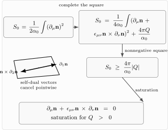
The two-derivative action can be written as a nonnegative square plus a topological term. Bound-saturating fields obey a first-order self-duality equation and have $S_0=4\pi |Q|/\alpha_0$.

The first-order equations are stronger than the ordinary field equation. This is why instantons are rare enough to be tractable, yet important enough to change the nonperturbative path integral.

CP¹ coordinates and holomorphic instantons

The target sphere is also the Riemann sphere $\mathbb{CP}^1$. Introduce the stereographic coordinate on the patch that omits the south pole,

$$w=\tan{\Theta\over2}\,e^{i\Phi}.$$

In terms of $w$,

$$\mathbf n={1\over1+|w|^2}\left(w+\bar w,-i(w-\bar w),1-|w|^2\right).$$

The omitted target point is represented by $w=\infty$ and is regular in the second coordinate $u=1/w$. Consequently, a pole of a rational function $w(z)$ is a coordinate pole, not a singularity of the physical unit vector $\mathbf n$.

The round metric on the target sphere is

$$d\mathbf n\cdot d\mathbf n={4\,dw\,d\bar w\over(1+|w|^2)^2}.$$

Consequently the action is

$$S_0 ={4\over\alpha_0}\int d^2x\, {\partial_z w\,\partial_{\bar z}\bar w+\partial_{\bar z}w\,\partial_z\bar w\over(1+|w|^2)^2},$$

and the topological charge is

$$Q ={1\over\pi}\int d^2x\, {\partial_z w\,\partial_{\bar z}\bar w-\partial_{\bar z}w\,\partial_z\bar w\over(1+|w|^2)^2}.$$

For a holomorphic map,

$$\partial_{\bar z}w=0,$$

we get

$$S_0={4\pi\over\alpha_0}Q, \qquad Q\ge0.$$

For an anti-holomorphic map,

$$\partial_z w=0,$$

we get

$$S_0={4\pi\over\alpha_0}|Q|, \qquad Q\le0.$$

Thus the instanton equation is just the Cauchy–Riemann equation in disguise. Instantons are holomorphic maps between Riemann spheres.

Since the boundary condition compactifies the domain to $S^2\simeq\mathbb C\cup\{\infty\}$, a smooth holomorphic instanton is a rational function,

$$w(z)={P(z)\over R(z)},$$

where $P$ and $R$ are polynomials with no common zero. Its degree is

$$Q=\max(\deg P,\deg R).$$

A convenient degree-$k$ family, when the zeros and poles do not cancel, is

$$w(z)=C\prod_{j=1}^k {z-a_j\over z-b_j}.$$

The points $a_j$ and $b_j$ are not particles sitting in spacetime. They are moduli of the rational map: they specify where the map takes the regular target values $w=0$ and $w=\infty$. Still, this zero–pole picture is a good way to remember how a multi-instanton map is assembled.

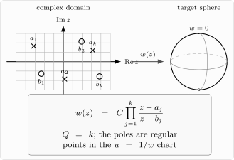
Holomorphic localized configurations are rational maps on the compactified complex plane. A degree-$k$ map has $Q=k$ and may be represented by zeros $a_j$ and coordinate poles $b_j$ of $w(z)$.

This holomorphic description is special to the $O(3)$ model. The general $O(N)$ model has important topology in other dimensions and for other target spaces, but this clean rational-map solution relies on

$$S^2\simeq\mathbb{CP}^1$$

and on two-dimensional conformal geometry.

The one-instanton profile

The simplest instanton is

$$w(z)=e^{i\chi}{z-z_0\over\rho},$$

where

$$z_0=X_1+iX_2, \qquad \rho>0, \qquad \chi\in[0,2\pi).$$

The real parameters have simple meanings:

• $z_0$ is the center of the instanton;
• $\rho$ is its size;
• $\chi$ is a residual target-space rotation around the boundary value.

This representative fixes the boundary value to $w(\infty)=\infty$, or $\mathbf n_\infty=(0,0,-1)$. Let $r=|z-z_0|$. Then

$$n^3(r)={\rho^2-r^2\over\rho^2+r^2},$$

so the center maps to the north pole, the circle $r=\rho$ maps to the equator, and infinity maps to the south pole. The topological charge density is

$$q(r)={\rho^2\over\pi(r^2+\rho^2)^2},$$

with

$$\int d^2x\,q(r)=1.$$

The Euclidean action density is

$$\mathcal L_E(r)={4\rho^2\over\alpha_0(r^2+\rho^2)^2},$$

and therefore

$$S_0={4\pi\over\alpha_0}.$$

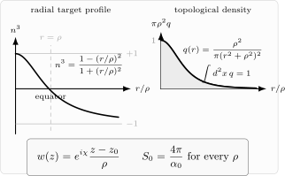
For $w=(z-z_0)/\rho$, the target polar angle obeys $\tan(\Theta/2)=r/\rho$. The size modulus $\rho$ sets where the profile crosses the target equator, but the total action remains $4\pi/\alpha_0$ for every $\rho$.

The independence of the classical action from $\rho$ is not an accident. The two-dimensional sigma model is classically scale invariant: under

$$x\mapsto \lambda x,$$

the measure $d^2x$ and the two derivatives in $(\partial\mathbf n)^2$ compensate exactly. The instanton can be large or small with the same classical cost.

Quantum mechanically the story is subtler. The coupling runs, so an RG-improved semiclassical estimate associates an instanton of size $\rho$ with a coupling evaluated near the momentum scale $1/\rho$:

$$e^{-4\pi/\alpha_0} \quad\leadsto\quad e^{-4\pi/\alpha(1/\rho)}.$$

The fluctuation determinant and collective-coordinate Jacobian supply additional powers of $\rho$; the replacement above isolates only the running exponential. This is also where the $O(3)$ model differs from a textbook double-well instanton. In quantum mechanics the instanton size is fixed by the potential. Here the classical two-dimensional action is scale invariant, so $\rho$ is a collective coordinate. The integration over $\rho$ is not a small technical detail; it tests the interface between semiclassics and the infrared strong-coupling region.

Small instantons are controlled by asymptotic freedom. Large instantons probe the strong-coupling infrared, where the model generates a mass scale. This is why instantons and the mass gap should not be mentally separated: the size integral forces the semiclassical saddle to talk to the RG.

Why instantons are nonperturbative

The instanton action is proportional to $1/\alpha_0$:

$$S_{\rm inst}={4\pi\over\alpha_0}.$$

Its contribution to the Euclidean path integral is therefore of the form

$$\exp\left(-{4\pi\over\alpha_0}\right).$$

No Taylor series in $\alpha_0$ around $\alpha_0=0$ can produce such a term. Perturbation theory expands inside the $Q=0$ sector; including instanton saddles adds the disconnected $Q\ne0$ sectors to the path integral. The small parameter is not a power of $\alpha_0$, but the exponentially small semiclassical weight.

For a dilute configuration of $k$ instantons and $\bar k$ anti-instantons, the leading semiclassical weight has the schematic form

$$\exp\left[-{4\pi\over\alpha_0}(k+\bar k)+i\theta(k-\bar k)\right],$$

before including the fluctuation determinants and interactions among collective coordinates. This formula is only schematic in the pure two-dimensional $O(3)$ model because the scale modulus explores strong coupling at large $\rho$. Still, it captures the essential lesson: topological sectors generate effects that are invisible in ordinary loop diagrams and carry theta-angle phases.

Summary

Localized configurations of the two-dimensional $O(3)$ sigma model with a fixed value at infinity define maps

$$S^2\to S^2,$$

and are classified by an integer degree $Q$. The topological charge can be written as

$$Q={1\over8\pi}\int d^2x\,\epsilon_{\mu\nu}\, \mathbf n\cdot(\partial_\mu\mathbf n\times\partial_\nu\mathbf n),$$

or as the pullback of the normalized area form on the target sphere. It is locally a total derivative, so a theta term does not modify the local classical equations, but it changes the relative phases of topological sectors.

The action obeys the Bogomolny bound

$$S_0\ge {4\pi\over\alpha_0}|Q|.$$

The bound is saturated by first-order self-dual equations. In stereographic coordinates, the $Q>0$ solutions are holomorphic maps $w=w(z)$, and compactness of the domain makes them rational functions. The one-instanton solution

$$w=e^{i\chi}{z-z_0\over\rho}$$

has action $4\pi/\alpha_0$, charge $1$, arbitrary center, arbitrary size, and a phase modulus. The size modulus is the doorway through which classical conformal invariance, asymptotic freedom, and infrared mass generation meet.

Common pitfalls

Inferring compactification from the action integral alone. The sector decomposition on $\mathbb R^2$ also uses a common limiting value $\mathbf n_\infty$. With a physical boundary or nonconstant asymptotic data, the degree and theta term require extra boundary information.

Dropping a local total derivative. The topological density can be written as $dA$ only patch by patch on the target sphere. Nonzero $Q$ is possible because the target area form is closed but not globally exact.

Treating a stereographic pole as a field singularity. The value $w=\infty$ is an ordinary point of $\mathbb{CP}^1$ and is covered by $u=1/w$. A pole of $w(z)$ can therefore be part of a perfectly smooth instanton.

Confusing instanton number with Noether charge. It is not generated by a continuous symmetry and does not count quanta. It is the degree of a map between compact oriented two-manifolds.

Assuming the size integral is automatically controlled. In the asymptotically free $O(3)$ model, small instantons are semiclassical, but large instantons feel the strongly coupled infrared. A dilute-gas formula without an infrared analysis is only schematic.

Dropping the factor of two in $Q$. Because $\epsilon_{\mu\nu}$ sums over both $(1,2)$ and $(2,1)$,

$${1\over8\pi}\epsilon_{\mu\nu}\mathbf n\cdot(\partial_\mu\mathbf n\times\partial_\nu\mathbf n) ={1\over4\pi}\mathbf n\cdot(\partial_1\mathbf n\times\partial_2\mathbf n).$$

Exercises

Exercise 1: the local total-derivative formula

Show that the topological charge density is locally a total derivative in target spherical coordinates:

$$q(x)={1\over4\pi}\epsilon_{\mu\nu}\sin\Theta\,\partial_\mu\Theta\,\partial_\nu\Phi ={1\over4\pi}\epsilon_{\mu\nu}\partial_\mu\left[(1-\cos\Theta)\partial_\nu\Phi\right].$$

Explain why this does not imply $Q=0$ for every smooth map.

Solution

Compute

$$\partial_\mu\left[(1-\cos\Theta)\partial_\nu\Phi\right] =\sin\Theta\,\partial_\mu\Theta\,\partial_\nu\Phi +(1-\cos\Theta)\partial_\mu\partial_\nu\Phi.$$

Contract with $\epsilon_{\mu\nu}$. The second term vanishes because $\partial_\mu\partial_\nu\Phi$ is symmetric in $\mu,\nu$ away from coordinate singularities, while $\epsilon_{\mu\nu}$ is antisymmetric. Thus

$$\epsilon_{\mu\nu}\partial_\mu\left[(1-\cos\Theta)\partial_\nu\Phi\right] =\epsilon_{\mu\nu}\sin\Theta\,\partial_\mu\Theta\,\partial_\nu\Phi.$$

This is only a local expression because $\Phi$ is not a globally smooth coordinate on $S^2$, and the one-form $(1-\cos\Theta)d\Phi$ is singular in the usual polar coordinate patch. A nonzero integral comes from the need to patch together local potentials on the target sphere. Equivalently, the normalized area form on $S^2$ is closed but not globally exact.

Exercise 2: deriving the Bogomolny bound

Derive the Bogomolny bound

$$S_0\ge {4\pi\over\alpha_0}|Q|$$

from the nonnegative square

$$\left(\partial_\mu\mathbf n+\epsilon_{\mu\nu}\mathbf n\times\partial_\nu\mathbf n\right)^2.$$

Solution

Using $\mathbf n^2=1$, we have $\mathbf n\cdot\partial_\mu\mathbf n=0$, and therefore

$$(\mathbf n\times\partial_\mu\mathbf n)^2=(\partial_\mu\mathbf n)^2.$$

Now expand the square and sum over $\mu$:

$$\left(\partial_\mu\mathbf n+\epsilon_{\mu\nu}\mathbf n\times\partial_\nu\mathbf n\right)^2 =2(\partial_\mu\mathbf n)^2 +2\epsilon_{\mu\nu}\partial_\mu\mathbf n\cdot(\mathbf n\times\partial_\nu\mathbf n).$$

The mixed product is

$$\partial_\mu\mathbf n\cdot(\mathbf n\times\partial_\nu\mathbf n) =-\mathbf n\cdot(\partial_\mu\mathbf n\times\partial_\nu\mathbf n).$$

Thus

$$\int d^2x\, \left(\partial_\mu\mathbf n+\epsilon_{\mu\nu}\mathbf n\times\partial_\nu\mathbf n\right)^2 =2\int d^2x\,(\partial_\mu\mathbf n)^2-16\pi Q.$$

Rearranging gives

$$S_0={1\over4\alpha_0}\int d^2x\, \left(\partial_\mu\mathbf n+\epsilon_{\mu\nu}\mathbf n\times\partial_\nu\mathbf n\right)^2 +{4\pi\over\alpha_0}Q.$$

For $Q>0$, the square is nonnegative, so $S_0\ge4\pi Q/\alpha_0$. Repeating the derivation with the opposite sign gives $S_0\ge -4\pi Q/\alpha_0$ for $Q<0$. Combining the two cases yields

$$S_0\ge {4\pi\over\alpha_0}|Q|.$$

Exercise 3: one-instanton charge density

For the one-instanton

$$w(z)={z\over\rho},$$

show that

$$q(r)={\rho^2\over\pi(r^2+\rho^2)^2},$$

and verify that $Q=1$.

Solution

For a holomorphic configuration,

$$q(x)={1\over\pi}{\partial_z w\,\partial_{\bar z}\bar w\over(1+|w|^2)^2}.$$

For $w=z/\rho$,

$$\partial_z w={1\over\rho}, \qquad \partial_{\bar z}\bar w={1\over\rho}, \qquad |w|^2={r^2\over\rho^2}.$$

Therefore

$$q(r) ={1\over\pi}{1/\rho^2\over(1+r^2/\rho^2)^2} ={\rho^2\over\pi(r^2+\rho^2)^2}.$$

Integrating in polar coordinates,

$$Q=\int d^2x\,q(r) =2\pi\int_0^\infty r\,dr\,{\rho^2\over\pi(r^2+\rho^2)^2} =2\rho^2\int_0^\infty {r\,dr\over(r^2+\rho^2)^2}.$$

Let $u=r^2+\rho^2$, so $du=2r\,dr$. Then

$$Q=\rho^2\int_{\rho^2}^{\infty}{du\over u^2}=1.$$

Exercise 4: a degree-k holomorphic map

Let

$$w(z)=\left({z\over\rho}\right)^k, \qquad k\in\mathbb Z_{>0}.$$

Use the fact that holomorphic maps saturate the Bogomolny bound to determine $Q$ and $S_0$. Give a geometric interpretation.

Solution

The function $w(z)=(z/\rho)^k$ is a degree-$k$ holomorphic map from the Riemann sphere to itself. A generic point in the target has $k$ preimages in the domain, counted with multiplicity. Hence

$$Q=k.$$

Because the map is holomorphic, it saturates the Bogomolny bound, so

$$S_0={4\pi k\over\alpha_0}.$$

Geometrically, the compactified Euclidean plane wraps the target sphere $k$ times with positive orientation. The map is not a collection of $k$ well-separated lumps for all moduli choices; it is a particularly symmetric degree-$k$ representative.

Exercise 5: stereographic poles are regular target points

Consider the rational map

$$w(z)={\rho\over z-z_0}.$$

Show that the apparent pole at $z=z_0$ is not a singularity of $\mathbf n$, determine its degree and topological charge, and identify the target value at the pole.

Solution

Near $z=z_0$, use the second target coordinate

$$u={1\over w}={z-z_0\over\rho}.$$

This coordinate is smooth and vanishes at $z=z_0$, so the map has no physical singularity there. In the unit-vector formula, $|w|\to\infty$ gives

$$\mathbf n\longrightarrow(0,0,-1),$$

the south pole of the target sphere. The rational map has numerator degree $0$ and denominator degree $1$, hence

$$Q=\deg(w)=1.$$

It is holomorphic as a map between Riemann spheres, even though one coordinate representation is meromorphic on the finite complex plane.

References

• Belavin, Alexander A., and Alexander M. Polyakov. “Metastable States of Two-Dimensional Isotropic Ferromagnets.” JETP Letters 22, no. 10 (1975): 245–247; Russian original, Pis’ma v ZhETF 22 (1975): 503–506.

Further reading

• Coleman, Sidney. Aspects of Symmetry: Selected Erice Lectures. Cambridge University Press, 1985.
• Fradkin, Eduardo. Field Theories of Condensed Matter Physics. 2nd ed. Cambridge University Press, 2013.
• Polyakov, Alexander M. Gauge Fields and Strings. Contemporary Concepts in Physics, Vol. 3. Harwood Academic Publishers, 1987.
• Zinn-Justin, Jean. Quantum Field Theory and Critical Phenomena. 5th ed. Oxford University Press, 2021.

References

Section titled “References”- Polyakov, Alexander M. Gauge Fields and Strings. Contemporary Concepts in Physics, vol. 3. Harwood Academic Publishers, 1987. DOI.