Nonlinear Sigma Models and Constraints

The previous pages used two-dimensional gauge theory as a laboratory for screening, confinement, bosonization, and charge lattices. We now move to a different but equally durable idea: the low-energy fields of a theory need not take values in a vector space. They may be constrained to live on a manifold.

The simplest example is a unit vector field

$$\mathbf n(x)=(n^1(x),\ldots,n^N(x)), \qquad \mathbf n^2(x)=1.$$

This is the $O(N)$ nonlinear sigma model. It describes maps from spacetime into the sphere $S^{N-1}$. The name “sigma model” is historical, but the idea is modern and unavoidable: whenever massive radial fluctuations are frozen and only angular Goldstone variables remain, the infrared theory is a field theory whose target space is a curved manifold.

The same structure appears in magnets, pion effective theories, string worldsheet dynamics, $CP^{N-1}$ models, large-$N$ methods, and many examples of dimensional transmutation. This page builds the model carefully: first from a linear field with a Mexican-hat potential, then as a constrained variational problem, then in local coordinates, and finally as a path integral with a Lagrange multiplier. The next page will use these preparations to compute the sigma-model beta function.

Helpful background. The Goldstone theorem and its pole argument explains why a vacuum manifold supplies massless angular variables, while dimensional transmutation and mass gaps supplies the RG language used near the end of this page. A nonlinear sigma model admits three complementary descriptions: a constrained field $\mathbf n^2=1$ with $N-1$ local degrees of freedom, a map $\mathbf n:M_d\to S^{N-1}$ whose target geometry enters the dynamics, and an effective theory obtained after massive radial modes are removed. These viewpoints are respectively convenient for variations, topology and beta functions, and applications to magnets and Goldstone modes.

From a linear model to a target space

Normalization used below. We work in Euclidean $d$ dimensions and write the $O(N)$ nonlinear sigma model as

$$S[\mathbf n] ={1\over 2\alpha_0}\int d^dx\,\partial_\mu\mathbf n\cdot\partial_\mu\mathbf n, \qquad \mathbf n^2=1.$$

The coupling has engineering dimension

$$[\alpha_0]=2-d.$$

Thus $\alpha_0$ is dimensionless in two dimensions. Some references absorb the factor of $1/2$ into $\alpha_0$; with that convention, several formulas below differ by a harmless factor of $2$.

Start with an $N$-component real scalar field

$$\boldsymbol\phi(x)=(\phi^1(x),\ldots,\phi^N(x))$$

with Euclidean action

$$S[\boldsymbol\phi] =\int d^dx\left[ {1\over2}\partial_\mu\boldsymbol\phi\cdot\partial_\mu\boldsymbol\phi +U(\boldsymbol\phi^2) \right].$$

Assume the potential has a minimum at nonzero radius,

$$\boldsymbol\phi^2=\rho_0^2, \qquad U'(\rho_0^2)=0.$$

It is then natural to write

$$\boldsymbol\phi(x)=\rho(x)\mathbf n(x), \qquad \mathbf n^2(x)=1.$$

Because

$$\mathbf n\cdot\partial_\mu\mathbf n ={1\over2}\partial_\mu(\mathbf n^2)=0,$$

the kinetic term separates cleanly:

$$\partial_\mu\boldsymbol\phi\cdot\partial_\mu\boldsymbol\phi =(\partial_\mu\rho)^2+\rho^2\partial_\mu\mathbf n\cdot\partial_\mu\mathbf n.$$

The radial field $\rho$ is massive if the curvature of $U$ at the minimum is nonzero. At distances much larger than the radial correlation length, one may integrate out $\rho$ and keep only the angular field $\mathbf n$. To leading order in derivatives,

$$\rho(x)=\rho_0+\text{massive fluctuations},$$

so the effective action becomes

$$S_{\rm eff}[\mathbf n] ={\rho_0^2\over2}\int d^dx\,\partial_\mu\mathbf n\cdot\partial_\mu\mathbf n+ \text{higher-derivative terms}.$$

Writing

$${1\over\alpha_0}=\rho_0^2$$

gives the nonlinear sigma-model form. More generally, integrating out the radial mode generates an infinite derivative expansion. If the matching coefficients $c_i$ are dimensionless, a convenient normalization is

$$\begin{aligned} S_{\rm eff}[\mathbf n] ={}&{1\over2\alpha_0}\int d^dx\,(\partial\mathbf n)^2\\ &+{c_1\over \alpha_0M_\rho^2} \int d^dx\,[(\partial\mathbf n)^2]^2\\ &+{c_2\over \alpha_0M_\rho^2} \int d^dx\,(\partial_\mu\mathbf n\cdot\partial_\nu\mathbf n)^2 +\cdots . \end{aligned}$$

Here $M_\rho$ is the radial mass. The factors of $1/(\alpha_0M_\rho^2)$ make the engineering dimensions explicit: each extra pair of derivatives costs two powers of the heavy scale. The two-derivative term is universal at low energy, whereas the $c_i$ remember details of the microscopic theory.

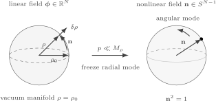
A linear $O(N)$ model with a potential minimum at $|\boldsymbol\phi|=\rho_0$ has a massive radial fluctuation and light angular modes. Freezing $\rho$ leaves a constrained field $\mathbf n\in S^{N-1}$.

This derivation is also the quickest way to understand what the coupling measures. A large radius $\rho_0$ means a stiff order parameter: gradients cost a lot of action, and $\alpha_0$ is small. A small radius means a flexible order parameter: angular fluctuations are cheap, and $\alpha_0$ is large. In perturbation theory, $\alpha_0$ is the strength of Goldstone scattering.

The derivative expansion also explains why the two-derivative sigma model is not an isolated miracle. It is the first term in a controlled low-energy series. The next page focuses on the running of the leading coupling $\alpha_0$, but higher-derivative operators are always present in the Wilsonian action. They are suppressed at long distance, not forbidden.

The sigma model as a map into a sphere

The field $\mathbf n(x)$ is a map

$$\mathbf n:M_d\longrightarrow S^{N-1},$$

where $M_d$ is Euclidean spacetime. The action is the Dirichlet energy of this map:

$$S[\mathbf n] ={1\over2\alpha_0}\int_{M_d} d^dx\,|d\mathbf n|^2.$$

At every spacetime point, the derivative $\partial_\mu\mathbf n$ is tangent to the sphere because

$$\mathbf n\cdot\partial_\mu\mathbf n=0.$$

Thus the theory does not describe $N$ independent scalar fields. It describes $N-1$ physical directions at each point, glued together nonlinearly as one moves over the sphere.

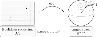
A nonlinear sigma-model field is a map from spacetime into a target manifold. For the $O(N)$ model the target is $S^{N-1}$, and local fluctuations are tangent to the sphere at $\mathbf n(x)$.

The same idea can be stated for a general target manifold $X$. If $q^A(x)$ are local coordinates on $X$ and $g_{AB}(q)$ is its metric, the two-derivative sigma-model action is

$$S[q] ={1\over2\alpha_0}\int d^dx\,g_{AB}(q)\partial_\mu q^A\partial_\mu q^B.$$

The sphere is the special case $X=S^{N-1}$ with the round metric. The coupling $\alpha_0$ controls the overall size of the target space in units of the spacetime cutoff. Curvature of the target space will become the source of renormalization on the next page.

Constrained variation and the equation of motion

Vary the action while preserving

$$\mathbf n^2=1.$$

An allowed variation $\delta\mathbf n$ obeys

$$\mathbf n\cdot\delta\mathbf n=0,$$

so it is tangent to the sphere. The first variation is

$$\delta S ={1\over\alpha_0}\int d^dx\,\partial_\mu\mathbf n\cdot\partial_\mu\delta\mathbf n.$$

After integrating by parts,

$$\delta S =-{1\over\alpha_0}\int d^dx\,\partial^2\mathbf n\cdot\delta\mathbf n,$$

where boundary terms are omitted. Since $\delta\mathbf n$ is any tangent vector, the tangent projection of $\partial^2\mathbf n$ must vanish:

$$P_T\partial^2\mathbf n=0, \qquad (P_T)^{ij}=\delta^{ij}-n^in^j.$$

Equivalently, $\partial^2\mathbf n$ must be normal to the sphere, hence proportional to $\mathbf n$. The proportionality factor is fixed by differentiating the constraint. First,

$$\mathbf n\cdot\partial_\mu\mathbf n=0.$$

Differentiating again and summing over $\mu$ gives

$$\mathbf n\cdot\partial^2\mathbf n +\partial_\mu\mathbf n\cdot\partial_\mu\mathbf n=0.$$

Therefore

$$\boxed{ \partial^2\mathbf n =-(\partial_\mu\mathbf n\cdot\partial_\mu\mathbf n)\mathbf n. }$$

This is the harmonic-map equation into the sphere. It is nonlinear even though the action contains only two derivatives. The nonlinearity is entirely due to the constraint.

A compact way to remember the equation is

$$P_T\partial^2\mathbf n=0, \qquad P_T=1-\mathbf n\mathbf n^T.$$

The Laplacian of the field need not vanish as a vector in $\mathbb R^N$; only its tangent part vanishes. This distinction is important when comparing sigma-model equations with free scalar equations. The normal component is fixed by the curvature of the target sphere.

A very useful equivalent formulation introduces a Lagrange multiplier $\lambda(x)$:

$$S[\mathbf n,\lambda] ={1\over2\alpha_0}\int d^dx\left[ \partial_\mu\mathbf n\cdot\partial_\mu\mathbf n +\lambda(\mathbf n^2-1) \right].$$

Varying $\lambda$ gives the constraint. Varying $\mathbf n$ gives

$$-\partial^2\mathbf n+\lambda\mathbf n=0,$$

or

$$\partial^2\mathbf n=\lambda\mathbf n.$$

Dotting with $\mathbf n$ and using $\mathbf n^2=1$ gives

$$\lambda=-(\partial_\mu\mathbf n)^2,$$

so the Lagrange-multiplier equation reproduces the constrained equation of motion.

For a real classical configuration, this equation fixes $\lambda=-(\partial\mathbf n)^2$; $\lambda$ is therefore not yet a positive mass squared. The mass interpretation used at large $N$ is a quantum saddle-point statement. In the exact Euclidean path integral the multiplier begins on an imaginary contour, and that contour can be deformed through a constant saddle $\lambda=m^2>0$, for which the quadratic operator is $-\partial^2+m^2$.

The role of $\lambda$ is analogous to pressure in an incompressible fluid. The pressure is not an independent propagating field in the simplest hydrodynamic description; it enforces the constraint $\nabla\cdot\mathbf v=0$. Here $\lambda$ enforces $\mathbf n^2=1$ and supplies precisely the normal force needed to keep the field on the sphere.

Local coordinates and derivative interactions

To do perturbation theory, choose a point on the sphere and coordinates near it. Around the “north pole,” write

$$\mathbf n=(\sigma,\boldsymbol\pi), \qquad \sigma=\sqrt{1-\boldsymbol\pi^2}, \qquad \boldsymbol\pi=(\pi^1,\ldots,\pi^{N-1}).$$

Then

$$\partial_\mu\sigma =-{\boldsymbol\pi\cdot\partial_\mu\boldsymbol\pi\over\sqrt{1-\boldsymbol\pi^2}},$$

and therefore

$$\partial_\mu\mathbf n\cdot\partial_\mu\mathbf n =\partial_\mu\boldsymbol\pi\cdot\partial_\mu\boldsymbol\pi +{(\boldsymbol\pi\cdot\partial_\mu\boldsymbol\pi)^2\over1-\boldsymbol\pi^2}.$$

The action becomes

$$S[\boldsymbol\pi] ={1\over2\alpha_0}\int d^dx\left[ (\partial_\mu\boldsymbol\pi)^2 +{(\boldsymbol\pi\cdot\partial_\mu\boldsymbol\pi)^2\over1-\boldsymbol\pi^2} \right].$$

Solving the constraint also changes the functional measure. In this patch the invariant sphere measure is, up to an overall constant,

$$[D\mathbf n]_{\mathbf n^2=1} = [D\boldsymbol\pi]\prod_x{1\over\sqrt{1-\boldsymbol\pi^2(x)}}.$$

With a momentum cutoff this Jacobian can contribute local terms, so a component calculation must keep it together with field renormalization. The covariant background-field method on the next page packages these effects without privileging a coordinate patch.

Expanding for small $\boldsymbol\pi$,

$$S[\boldsymbol\pi] ={1\over2\alpha_0}\int d^dx\left[ (\partial\boldsymbol\pi)^2 +(\boldsymbol\pi\cdot\partial\boldsymbol\pi)^2 +\boldsymbol\pi^2(\boldsymbol\pi\cdot\partial\boldsymbol\pi)^2+ \cdots \right].$$

If we introduce canonically normalized fields

$$\boldsymbol\pi=\sqrt{\alpha_0}\,\boldsymbol\varphi,$$

then

$$S[\boldsymbol\varphi] ={1\over2}\int d^dx\,(\partial\boldsymbol\varphi)^2 +{\alpha_0\over2}\int d^dx\,(\boldsymbol\varphi\cdot\partial\boldsymbol\varphi)^2 +O(\alpha_0^2).$$

This displays two key facts. First, the particles are massless in perturbation theory: there is no potential term for $\boldsymbol\varphi$. Second, the interactions are derivative interactions, so amplitudes vanish when external momenta are taken soft. The coupling $\alpha_0$ is the expansion parameter for scattering.

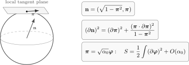
A coordinate patch solves the constraint locally. Near a chosen pole, $\mathbf n=(\sqrt{1-\boldsymbol\pi^2},\boldsymbol\pi)$, and the round metric produces derivative self-interactions for the $N-1$ Goldstone coordinates $\boldsymbol\pi$.

For $S^2$, ordinary spherical coordinates give the same structure:

$$\mathbf n=(\sin\theta\cos\phi,\sin\theta\sin\phi,\cos\theta),$$

so

$$(\partial\mathbf n)^2=(\partial\theta)^2+ \sin^2\theta\,(\partial\phi)^2.$$

This form is geometrically transparent but not globally nonsingular: the coordinate $\phi$ degenerates at the poles. The vector constraint $\mathbf n^2=1$ avoids this coordinate singularity at the cost of introducing a redundant variable and a constraint.

The one-dimensional case: the quantum rotor

The sigma model in one Euclidean dimension is ordinary quantum mechanics on a sphere:

$$S={1\over2\alpha_0}\int dt\,\dot{\mathbf n}^2, \qquad \mathbf n^2=1.$$

This is a rigid rotor with moment of inertia

$$I={1\over\alpha_0}.$$

The Hamiltonian is the Laplacian on $S^{N-1}$,

$$H=-{\alpha_0\over2}\Delta_{S^{N-1}}.$$

The eigenvalues of $-\Delta_{S^{N-1}}$ are

$$\ell(\ell+N-2), \qquad \ell=0,1,2,\ldots.$$

Thus

$$\boxed{ E_\ell={\alpha_0\over2}\ell(\ell+N-2). }$$

For $S^2$, this becomes

$$E_\ell={\alpha_0\over2}\ell(\ell+1).$$

The ground state is the constant wavefunction on the sphere. It is fully $O(N)$ invariant. There is no spontaneous choice of direction in finite-dimensional quantum mechanics, and the first excited state is separated by a finite gap. This is the simplest warning that “Goldstone coordinates” are not automatically physical massless particles in every dimension and volume. Infrared fluctuations matter.

In $d>2$, the coupling $\alpha_0$ has negative engineering dimension and long-distance fluctuations can be weak in an ordered phase. In $d=2$, $\alpha_0$ is classically marginal; quantum fluctuations accumulate logarithmically and eventually generate a scale. That logarithm is the subject of the next page.

Coordinate patches and what perturbation theory misses

The local coordinate field $\boldsymbol\pi$ covers only one patch of the sphere. Perturbation theory around $\boldsymbol\pi=0$ is therefore an expansion around maps whose image stays near one point on the target. That is exactly what is wanted for short-distance beta functions, but it cannot see configurations that wrap the whole sphere.

This warning will matter in Sigma-Model Instantons and Topological Charge. For $O(3)$ in two Euclidean dimensions, finite-action configurations are maps $S^2\to S^2$ with integer winding number. Those sectors are invisible in any finite Taylor expansion in $\boldsymbol\pi$ around a constant field.

Enforcing the constraint in the path integral

The constrained path integral may be written schematically as

$$Z=\int [D\mathbf n]\,\prod_x\delta(\mathbf n^2(x)-1) \exp\left[-{1\over2\alpha_0}\int d^dx\,(\partial\mathbf n)^2\right].$$

Using a Lagrange multiplier,

$$\prod_x\delta(\mathbf n^2(x)-1) \sim \int [D\lambda]\, \exp\left[-{1\over2\alpha_0}\int d^dx\,\lambda(\mathbf n^2-1)\right],$$

where the exact contour for $\lambda$ is chosen so that the integral represents a delta function. In saddle-point and Euclidean perturbation theory one usually deforms this contour to a steepest-descent contour. The practical representation is

$$Z=\int [D\mathbf n][D\lambda]\, \exp\left[-{1\over2\alpha_0}\int d^dx\, \big((\partial\mathbf n)^2+\lambda(\mathbf n^2-1)\big) \right].$$

This formulation is especially useful for large-$N$ expansions. Integrating out the $N$ components of $\mathbf n$ gives an effective action for $\lambda$; after the contour deformation just described, a constant saddle $\lambda=m^2$ behaves like a dynamically generated mass. The large-N saddle point develops that argument after the perturbative beta-function calculation.

A first Wilsonian look at the constraint

Even before computing the full beta function, one can see why the nonlinear sigma model renormalizes. Split the field into a slowly varying background and short-wavelength tangent fluctuations. A convenient local parameterization is

$$\mathbf n(x) =\sqrt{1-\boldsymbol\xi^2(x)}\,\mathbf n_0(x) +\xi^a(x)\mathbf e_a(x),$$

where

$$\mathbf n_0^2=1, \qquad \mathbf n_0\cdot\mathbf e_a=0, \qquad \mathbf e_a\cdot\mathbf e_b=\delta_{ab}, \qquad a=1,\ldots,N-1.$$

The fields $\xi^a$ are tangent fluctuations. At leading order around a slowly varying background, their Gaussian action is

$$S_{\rm fast} \simeq {1\over2\alpha_0}\int d^dx\,\partial_\mu\xi^a\partial_\mu\xi^a.$$

Therefore, in momentum space,

$$\langle \xi^a(k)\xi^b(-k)\rangle =\alpha_0{\delta^{ab}\over k^2}.$$

In two dimensions, the fluctuation in a thin momentum shell

$$\Lambda'<|k|<\Lambda$$

is logarithmic:

$$\begin{aligned} \langle \boldsymbol\xi^2(x)\rangle_{\rm shell} &=(N-1)\alpha_0 \int_{\Lambda'<|k|<\Lambda}{d^2k\over(2\pi)^2}{1\over k^2}\\ &={(N-1)\alpha_0\over2\pi}\log{\Lambda\over\Lambda'}. \end{aligned}$$

The square root in the parameterization gives

$$\sqrt{1-\boldsymbol\xi^2} =1-{1\over2}\boldsymbol\xi^2+\cdots,$$

so averaging over short modes changes the length of the slow field:

$$\langle\mathbf n(x)\rangle_{\rm fast} =\left(1-{1\over2}\langle\boldsymbol\xi^2\rangle_{\rm shell}+\cdots\right)\mathbf n_0(x).$$

But the final low-energy field must again be a unit vector. Therefore the Wilsonian step contains a field rescaling. At the same time, integrating out the shell changes the coefficient of

$$\int d^2x\,(\partial\mathbf n_0)^2.$$

These two effects combine into the beta function. The full coefficient is not simply the $(N-1)$ appearing in $\langle\boldsymbol\xi^2\rangle$; the geometry of parallel transport on the sphere also matters. The next page computes the result and shows why the two-dimensional $O(N)$ model is asymptotically free for $N>2$.

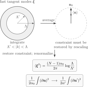
A Wilsonian step integrates tangent fluctuations $\boldsymbol\xi$ in the shell $\Lambda'<|k|<\Lambda$. Because the target-space constraint must be restored after averaging, the shell renormalizes both the field normalization and the stiffness $1/\alpha$.

Summary

A nonlinear sigma model is an effective field theory of maps into a target manifold. For the $O(N)$ model, the field is a unit vector $\mathbf n\in S^{N-1}$ and the leading Euclidean action is

$$S={1\over2\alpha_0}\int d^dx\,(\partial\mathbf n)^2, \qquad \mathbf n^2=1.$$

It arises naturally from a linear model when the radial mode is massive and frozen. The constraint makes the theory nonlinear even though the action has only two derivatives. The equation of motion is

$$\partial^2\mathbf n=-(\partial\mathbf n)^2\mathbf n,$$

or equivalently $P_T\partial^2\mathbf n=0$.

Local coordinates solve the constraint but introduce derivative self-interactions. After canonical normalization, the coupling $\alpha_0$ controls Goldstone scattering. In one dimension the model is a quantum rotor with a unique symmetric ground state. In two dimensions the coupling is classically marginal, and short-distance tangent fluctuations produce logarithms. The next step is to compute how those logarithms change $\alpha_0$.

Common pitfalls

Confusing spacetime dimension and target-space dimension. The symbol $d$ counts Euclidean spacetime dimensions. The symbol $N$ counts components of $\mathbf n$, so the target is $S^{N-1}$.

Treating the $N$ components of $\mathbf n$ as independent. The constraint removes one degree of freedom at each point. Perturbation theory must use tangent fluctuations or a Lagrange multiplier.

Thinking the absence of a potential means a free theory. The two-derivative action is nonlinear because the target-space metric is curved. In local coordinates, the interactions are derivative interactions.

Using one coordinate patch globally. Coordinates such as $\boldsymbol\pi$ or $(\theta,\phi)$ are local. The vector constraint is often safer for global questions, topology, and instantons.

Applying Goldstone’s theorem without checking infrared physics. The sigma model describes Goldstone variables perturbatively, but in low dimensions quantum fluctuations can destroy long-range order and generate a mass gap.

Exercises

Exercise 1: radial and angular kinetic terms

Let

$$\boldsymbol\phi(x)=\rho(x)\mathbf n(x), \qquad \mathbf n^2=1.$$

Show that

$$(\partial_\mu\boldsymbol\phi)^2 =(\partial_\mu\rho)^2+ \rho^2(\partial_\mu\mathbf n)^2.$$

Use this to identify the leading sigma-model coupling when $\rho$ is frozen at $\rho_0$.

As a tree-level matching check, take

$$U(\rho^2)=U(\rho_0^2)+{1\over2}M_\rho^2(\rho-\rho_0)^2+\cdots$$

and neglect derivatives of the heavy fluctuation $s=\rho-\rho_0$. Solve for $s$ through order $(\partial\mathbf n)^2$ and find the induced $[(\partial\mathbf n)^2]^2$ term.

Solution

Differentiate

$$\partial_\mu\boldsymbol\phi =(\partial_\mu\rho)\mathbf n+ \rho\partial_\mu\mathbf n.$$

Squaring gives

$$(\partial_\mu\boldsymbol\phi)^2 =(\partial_\mu\rho)^2\mathbf n^2 +2\rho(\partial_\mu\rho)\mathbf n\cdot\partial_\mu\mathbf n +\rho^2(\partial_\mu\mathbf n)^2.$$

Since $\mathbf n^2=1$,

$$\mathbf n\cdot\partial_\mu\mathbf n={1\over2}\partial_\mu(\mathbf n^2)=0.$$

Therefore

$$(\partial_\mu\boldsymbol\phi)^2 =(\partial_\mu\rho)^2+ \rho^2(\partial_\mu\mathbf n)^2.$$

If $\rho=\rho_0$ at low energy, the kinetic term becomes

$${\rho_0^2\over2}\int d^dx\,(\partial\mathbf n)^2.$$

Comparing with

$${1\over2\alpha_0}\int d^dx\,(\partial\mathbf n)^2$$

gives

$$\alpha_0={1\over\rho_0^2}$$

in this normalization.

For the matching calculation, abbreviate $X=(\partial\mathbf n)^2$. Through order $X^2$, the terms that depend on $s$ are

$$\mathcal L_s =\rho_0sX+{1\over2}M_\rho^2s^2+O(X^3),$$

where terms with derivatives on $s$ are higher order in the heavy-mass expansion.

The algebraic heavy-field equation gives

$$s=-{\rho_0\over M_\rho^2}X+O(X^2).$$

Substitution yields

$$\mathcal L_{\rm eff} ={\rho_0^2\over2}X -{\rho_0^2\over2M_\rho^2}X^2+\cdots ={1\over2\alpha_0}X -{1\over2\alpha_0M_\rho^2}X^2+\cdots .$$

This simple ultraviolet completion therefore has $c_1=-1/2$ in the normalization used above. Other microscopic interactions change the dimensionless matching coefficients but not the suppression by $M_\rho^{-2}$.

Exercise 2: constrained equation of motion

Starting from

$$S[\mathbf n,\lambda] ={1\over2\alpha_0}\int d^dx\left[(\partial\mathbf n)^2+ \lambda(\mathbf n^2-1)\right],$$

derive the constrained equation of motion

$$\partial^2\mathbf n=-(\partial\mathbf n)^2\mathbf n.$$

Solution

Varying with respect to $\lambda$ gives

$$\mathbf n^2=1.$$

Varying with respect to $\mathbf n$ gives

$$\delta S ={1\over\alpha_0}\int d^dx\left[ \partial_\mu\mathbf n\cdot\partial_\mu\delta\mathbf n+ \lambda\mathbf n\cdot\delta\mathbf n \right].$$

After integrating by parts,

$$\delta S ={1\over\alpha_0}\int d^dx\left[-\partial^2\mathbf n+ \lambda\mathbf n\right]\cdot\delta\mathbf n.$$

Thus

$$\partial^2\mathbf n=\lambda\mathbf n.$$

Dot with $\mathbf n$:

$$\mathbf n\cdot\partial^2\mathbf n=\lambda.$$

Differentiating the constraint twice gives

$$\mathbf n\cdot\partial^2\mathbf n=-(\partial\mathbf n)^2.$$

Therefore

$$\lambda=-(\partial\mathbf n)^2,$$

and hence

$$\partial^2\mathbf n=-(\partial\mathbf n)^2\mathbf n.$$

Exercise 3: local-coordinate interaction

Use the local parameterization

$$\mathbf n=(\sqrt{1-\boldsymbol\pi^2},\boldsymbol\pi)$$

to show that

$$(\partial\mathbf n)^2 =(\partial\boldsymbol\pi)^2+{(\boldsymbol\pi\cdot\partial\boldsymbol\pi)^2\over1-\boldsymbol\pi^2}.$$

Then rescale $\boldsymbol\pi=\sqrt{\alpha_0}\boldsymbol\varphi$ and find the first interaction term.

Solution

Let

$$\sigma=\sqrt{1-\boldsymbol\pi^2}.$$

Then

$$\partial_\mu\sigma =-{\boldsymbol\pi\cdot\partial_\mu\boldsymbol\pi\over\sqrt{1-\boldsymbol\pi^2}}.$$

Therefore

$$(\partial\mathbf n)^2 =(\partial\sigma)^2+(\partial\boldsymbol\pi)^2 =(\partial\boldsymbol\pi)^2+ {(\boldsymbol\pi\cdot\partial\boldsymbol\pi)^2\over1-\boldsymbol\pi^2}.$$

The action is

$$S={1\over2\alpha_0}\int d^dx\left[(\partial\boldsymbol\pi)^2+ (\boldsymbol\pi\cdot\partial\boldsymbol\pi)^2+O(\boldsymbol\pi^6) \right].$$

With

$$\boldsymbol\pi=\sqrt{\alpha_0}\boldsymbol\varphi,$$

we get

$$S={1\over2}\int d^dx\,(\partial\boldsymbol\varphi)^2 +{\alpha_0\over2}\int d^dx\,(\boldsymbol\varphi\cdot\partial\boldsymbol\varphi)^2 +O(\alpha_0^2).$$

Thus the first interaction is a four-field derivative interaction proportional to $\alpha_0$.

Exercise 4: quantum-rotor spectrum

For the one-dimensional model

$$S={1\over2\alpha_0}\int dt\,\dot{\mathbf n}^2, \qquad \mathbf n\in S^{N-1},$$

show that the energy levels are

$$E_\ell={\alpha_0\over2}\ell(\ell+N-2).$$

What is the gap above the ground state?

Solution

The action is that of a particle moving on the unit sphere with moment of inertia

$$I={1\over\alpha_0}.$$

The quantum Hamiltonian is

$$H=-{1\over2I}\Delta_{S^{N-1}} =-{\alpha_0\over2}\Delta_{S^{N-1}}.$$

Scalar spherical harmonics on $S^{N-1}$ obey

$$-\Delta_{S^{N-1}}Y_\ell=\ell(\ell+N-2)Y_\ell, \qquad \ell=0,1,2,\ldots.$$

Therefore

$$E_\ell={\alpha_0\over2}\ell(\ell+N-2).$$

The ground state has $\ell=0$, so $E_0=0$ in this normalization. The first excited level has $\ell=1$, so

$$\Delta E=E_1-E_0={\alpha_0\over2}(N-1).$$

The finite gap reflects the absence of spontaneous symmetry breaking in finite-dimensional quantum mechanics.

Exercise 5: the two-dimensional shell logarithm

Compute the two-dimensional shell integral

$$I_{\rm shell}=\int_{\Lambda'<|k|<\Lambda}{d^2k\over(2\pi)^2}{1\over k^2}.$$

Use it to find $\langle\boldsymbol\xi^2\rangle_{\rm shell}$ for $N-1$ tangent fields with propagator $\alpha_0/k^2$.

Solution

In polar coordinates,

$$d^2k=k\,dk\,d\theta.$$

Therefore

$$I_{\rm shell} ={1\over(2\pi)^2}\int_0^{2\pi}d\theta\int_{\Lambda'}^{\Lambda}{k\,dk\over k^2} ={1\over2\pi}\int_{\Lambda'}^{\Lambda}{dk\over k}.$$

Thus

$$I_{\rm shell}={1\over2\pi}\log{\Lambda\over\Lambda'}.$$

For $N-1$ tangent fields,

$$\langle\boldsymbol\xi^2\rangle_{\rm shell} =\sum_{a=1}^{N-1}\langle\xi^a(x)\xi^a(x)\rangle =(N-1)\alpha_0 I_{\rm shell}.$$

Hence

$$\langle\boldsymbol\xi^2\rangle_{\rm shell} ={(N-1)\alpha_0\over2\pi}\log{\Lambda\over\Lambda'}.$$

This is the elementary logarithm behind the Wilsonian renormalization of the two-dimensional sigma model.

References

• A. M. Polyakov, “Interaction of Goldstone Particles in Two Dimensions. Applications to Ferromagnets and Massive Yang–Mills Fields,” Physics Letters B 59 (1975) 79–81, doi:10.1016/0370-2693(75)90161-6.

Further reading

• S. Coleman, Lectures of Sidney Coleman on Quantum Field Theory, edited by B. G. Chen et al., World Scientific, Singapore, 2019.
• A. M. Polyakov, Gauge Fields and Strings, Contemporary Concepts in Physics, Vol. 3, Harwood Academic Publishers, Chur, 1987.
• S. Weinberg, The Quantum Theory of Fields, Volume II: Modern Applications, Cambridge University Press, Cambridge, 1996.
• A. Zee, Quantum Field Theory in a Nutshell, 2nd ed., Princeton University Press, Princeton, 2010.
• J. Zinn-Justin, Quantum Field Theory and Critical Phenomena, 5th ed., Oxford University Press, Oxford, 2021.