

Spectral Representation and Dispersion Integrals
The previous lesson on causality, commutators, and support explained why the commutator of two local scalar fields vanishes outside the light cone, even though the Feynman propagator itself does not. This page turns that causal statement into an analytic one. The same two-point function that describes propagation in spacetime becomes, after Fourier transform, a function of complex energy or complex invariant momentum. Poles, branch cuts, and prescriptions are not optional decorations; they encode the spectrum of the theory.
The main lesson is that an exact two-point function is a spectral average of free propagators with all allowed invariant masses, with local subtraction terms when the time-ordered product requires them. A stable one-particle state isolated from the continuum gives an isolated pole. Multiparticle states give a continuum. The discontinuity across the continuum cut determines a nonnegative spectral density, and analytic functions with such cuts obey dispersion relations: under the growth conditions developed below, their real parts are reconstructible from their imaginary parts up to subtraction constants.
This is the bridge from the causal spacetime picture to the momentum-space picture used in scattering theory and renormalization. It also prepares Thresholds, Cuts, and Imaginary Parts, where thresholds and imaginary parts are read directly from the phase space of intermediate states.
Here is the reader’s dictionary for this page:
| Spectral feature | Momentum-space singularity | Physical meaning |
|---|---|---|
| simple pole at | stable one-particle state created by the field | |
| branch cut beginning at | continuum of multiparticle states | |
| jump across the cut | on-shell intermediate states | |
| subtraction polynomial | analytic ambiguity | local counterterms or renormalization conditions |
The table is deliberately phrased in both analytic and physical language. A spectral representation is useful precisely because it lets one translate between them.
Wightman functions as boundary values
Section titled “Wightman functions as boundary values”The spectral representation follows by inserting physical intermediate states. For its completeness and positivity assumptions, see Spectral Decomposition of Two-Point Functions. Lorentzian Boundary Conditions and iε fixes the prescription conventions, while Subtracted Dispersion Relations develops the additional hypotheses required for scattering-amplitude applications.
Start with the free real scalar field
The positive-frequency Wightman function is
This integral is not an ordinary function everywhere; it is a distribution. The correct definition is obtained by giving time a small negative imaginary part,
so that positive-energy modes are slightly damped:
The reversed ordering is the opposite boundary value:
which is obtained with . Thus the two Wightman functions are boundary values of the same analytic object from opposite sides.
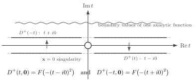
Positive-energy propagation selects a boundary value in complex time. The ordering is obtained by , while the reversed ordering is obtained by . The time-ordered propagator glues these boundary values together.
The time-ordered two-point function is therefore
Equivalently,
The in momentum space is the same boundary-value information as the prescription in coordinate space. Positive-energy modes propagate forward in the time-ordered product, while negative-energy poles are placed on the opposite side of the contour.
The massless coordinate-space singularity
Section titled “The massless coordinate-space singularity”For a massless scalar in four spacetime dimensions, the positive-frequency integral can be evaluated explicitly:
The reversed ordering is
The light cone is the singular surface. For ,
The elementary distribution identity
then explains why the massless commutator is supported on the light cone. The singularity is not a bug in the propagator. It is the analytic shadow of sharp relativistic propagation.
In spacetime dimensions, dimensional analysis gives the leading massless short-distance behavior
Equivalently, a free scalar field has engineering dimension
In the exponent vanishes and this formula must be replaced by a logarithm; the massless scalar also has an infrared zero-mode ambiguity. The engineering dimension is still zero, but dimensional analysis alone does not determine the logarithm.
This short-distance power will later reappear in renormalization: loop divergences are the momentum-space version of coincident-point singularities.
Inserting a complete set of states
Section titled “Inserting a complete set of states”The free result is only the beginning. Assume a positive physical Hilbert-space metric and the forward-cone spectrum condition. The chosen Poincaré-invariant vacuum is the unique translation-invariant state in this representation. Let be a Hermitian scalar Heisenberg operator with a well-defined two-point distribution, and remove its vacuum expectation value by defining
Translation invariance gives
Insert a complete set of exact energy-momentum eigenstates between the two fields:
Every term has positive energy, , and invariant mass squared . Lorentz invariance allows us to group the states by their invariant mass squared . This defines a nonnegative spectral density such that
where is the free Wightman function for a scalar particle of mass :
The positivity is crucial:
It follows directly from the squared matrix elements in the positive-metric Hilbert space Schwartz 2014, § 24.2.1, pp. 467–469. Without the vacuum subtraction, a nonzero one-point function would add a disconnected constant in position space, or a term proportional to in momentum space; it is not part of the propagating spectral measure discussed here.
One should read as a positive measure, not necessarily as a smooth function. Isolated particles appear as delta functions in this measure. Continua appear as ordinary functions beginning at thresholds. Writing both with the same symbol is what makes the pole-plus-cut structure look so simple.
In the unsubtracted regime specified above, the time-ordered version is the Källén–Lehmann representation:
where
In momentum space,
This formula says that the exact propagator is a superposition of free propagators. The interactions have not disappeared; they are encoded in .
Poles, continua, and the meaning of the spectral density
Section titled “Poles, continua, and the meaning of the spectral density”Suppose has nonzero overlap with a stable one-particle state of physical mass . Then the spectral density contains a delta function:
Use the standard relativistic one-particle normalization
Then the matrix element
defines the pole residue; Lorentz invariance makes this scalar matrix element momentum independent. The number measures how strongly the field creates the physical one-particle state from the vacuum. The propagator contains
The continuum part begins at the lightest multiparticle threshold accessible to . For example, suppose an unbroken symmetry makes the field and a stable scalar of mass odd, and there is no additional stable species or bound state below . The invariant vacuum is even, so two copies of this scalar cannot contribute in the odd channel. The first kinematically allowed multiparticle channel then consists of three copies, with threshold
The spectral continuum starts there when this channel has nonzero weight arbitrarily close to threshold. For a free elementary field, these three-particle matrix elements vanish, so there is no such continuum. Additional stable species require checking the allowed channels again: an odd-plus-even pair can lower this threshold while preserving the symmetry. Without a selection rule, two particles of mass can instead give a threshold at .
For a canonically normalized elementary field with a well-defined canonical equal-time commutator and finite total spectral weight, that commutator fixes the sum rule
The inequality follows because the remaining continuum weight is nonnegative. A rescaled field or a composite operator has no unit normalization sum rule. Moreover, time-ordered correlators of composite operators can require local contact terms, which appear as subtraction polynomials in momentum space in addition to their spectral part.
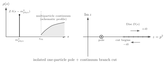
A stable particle with nonzero field overlap contributes a delta function to ; when its mass is separated from the continuum, the propagator has an isolated pole. The illustrated multiparticle continuum has nonzero spectral weight arbitrarily close to its threshold , where the branch cut begins.
The pole is a particle. The cut is a continuum of possible intermediate states. A spectral density is therefore a bookkeeping device for what the field can create.
Discontinuities and imaginary parts
Section titled “Discontinuities and imaginary parts”Let the analytic function off its cut be
Away from the real positive axis, is analytic. On the cut,
Thus
This is the simplest form of the rule that an imaginary part measures the density of physical intermediate states. The minus sign comes directly from approaching the kernel from the upper half-plane:
For the full Feynman propagator itself,
the entire spectral measure—isolated delta functions and continuum density—appears distributionally in its real part:
Multiplying by the extracted factor rotates the imaginary part of into the real part of . This is one reason signs in spectral formulas can look different across textbooks. The invariant content is the same: the discontinuity across the physical cut is fixed by the positive spectral density.
Dispersion integrals
Section titled “Dispersion integrals”The spectral representation is a special case of a more general complex-analysis statement. Let be analytic in the complex -plane except for a cut beginning at , and suppose is real analytic:
If falls sufficiently fast at infinity, Cauchy’s theorem gives
This is an unsubtracted dispersion relation. The discontinuity on the cut determines the whole function.
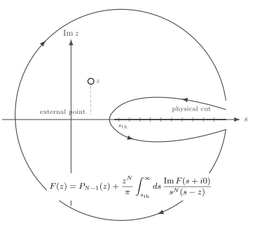
Cauchy’s theorem expresses an analytic function in terms of its discontinuity along the physical cut. If the large circle does not vanish, one subtracts enough polynomial terms to make the contour integral convergent.
Many QFT functions do not fall fast enough at infinity. Then one subtracts at a point away from the cut:
If , the origin is an allowed subtraction point and this becomes
With subtractions at the origin (again assuming it lies off the cut),
Here is a polynomial of degree at most . Its physical interpretation depends on which function is being reconstructed. A polynomial added to a connected two-point correlator Fourier transforms to a contact distribution, a sum of derivatives of . Where such local ambiguities are allowed, they can be represented by local quadratic source terms such as and . They do not change the correlator at separated points.
By contrast, mass and kinetic counterterms in the field action are local terms in the inverse propagator, or equivalently in its 1PI self-energy:
They do not add a polynomial directly to the full propagator. For example, with its overall Feynman factor removed and away from the pole,
The mass insertion gives a double denominator, not a constant. Thus one must specify whether denotes a correlator or a proper two-point function before identifying its subtraction coefficients with action parameters. The subtracted-dispersion treatment develops the subtraction data and high-energy assumptions independently of this choice of application.
So the dispersion relation packages two ideas together:
- the nonlocal part of the amplitude is controlled by physical intermediate states;
- the remaining ambiguity is local and must be fixed by renormalization conditions.
This separates the discontinuity, fixed by the spectrum and matrix elements, from local subtraction data. The polynomial must be fixed by conditions on the specified function; these may be action-parameter renormalization conditions or conditions on local source/contact terms.
Self-energy and spectral cuts
Section titled “Self-energy and spectral cuts”For a scalar field, the exact propagator can also be written in Dyson form,
where is the self-energy. The spectral representation applies to the full propagator, while dispersion relations apply to or to any other 1PI function with the appropriate analytic properties.
At low order, a self-energy graph becomes nonanalytic when its internal lines can simultaneously go on shell. This is the origin of branch cuts. In a theory, the tadpole shifts the mass but has no external-momentum cut. The first momentum-dependent scalar self-energy appears in the two-loop sunset diagram, schematically
The denominator can become singular when the three internal particles are simultaneously on shell and carry total momentum . This is the three-particle threshold.
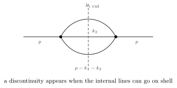
A self-energy diagram develops a discontinuity when the dashed cut can pass through internal lines that are all on shell. The cut is the diagrammatic image of the multiparticle continuum in the spectral representation.
The time-domain picture makes the same point. If a field can create intermediate states with energies , then its correlator contains terms of the form
A single isolated energy gives a pure exponential and hence a pole after Fourier transform. A continuum of energies gives an integral over exponentials, and that integral produces a branch cut. Thresholds, Cuts, and Imaginary Parts uses this idea to extract threshold behavior from nonrelativistic phase space near the onset of a multiparticle continuum.
Euclidean viewpoint
Section titled “Euclidean viewpoint”For spacelike momentum, write
In the same unsubtracted regime, the Euclidean two-point function has a positive denominator,
With the earlier Lorentzian definition , this Euclidean object corresponds to the positive continuation after stripping the overall Lorentzian factor. This minus sign is pure bookkeeping; the useful fact is that is real and positive if .
The Euclidean form shows why Euclidean correlation functions are often cleaner: the poles and cuts are not crossed, and the spectral density appears through a smooth kernel.
At large Euclidean momentum,
provided the moments are sufficiently well behaved. This expansion is a first glimpse of the short-distance logic behind the operator product expansion: high Euclidean momentum probes moments of spectral data and local short-distance structure.
Summary
Section titled “Summary”The two-point function of an interacting scalar field has three equivalent descriptions. In spacetime, it is a boundary value of an analytic function, with prescriptions selecting how singularities are approached. In the Hilbert space, it is a sum over exact intermediate states. In momentum space, it is an analytic function with poles and cuts.
In the unsubtracted regime, the Källén–Lehmann representation is the synthesis:
A stable particle isolated from the continuum gives an isolated pole. A multiparticle continuum gives a branch cut whose discontinuity determines the spectral density. Dispersion relations reconstruct analytic functions from their discontinuities, up to subtraction polynomials fixed by local normalization conditions.
Common pitfalls
Section titled “Common pitfalls”Confusing the Feynman propagator with a positive spectral function. The positivity belongs to , which comes from squared matrix elements. The time-ordered propagator contains extra factors of and principal values.
Forgetting the boundary value. Expressions such as or are incomplete as distributions. The prescription says which side of the singular surface is meant.
Thinking every imaginary part means instability. A cut in a two-point function may simply mean that the field can create multiparticle states. An unstable particle is more subtle: its pole moves away from the real axis on a second sheet.
Ignoring subtraction constants. Dispersion integrals often require subtractions. The subtraction constants are physical renormalization data, not optional nuisances.
Treating as smooth by default. A stable particle contributes a delta function, not a narrow smooth bump. A resonance is different: it is associated with a pole on another sheet and appears as structure in the continuum.
Exercises
Section titled “Exercises”Exercise 1
Section titled “Exercise 1”Evaluate the massless positive-frequency Wightman function in four spacetime dimensions:
Show that
Solution
Let . The angular integral is
Thus
So
Using
we get
This simplifies to
Therefore
Taking gives the stated boundary value.
Exercise 2
Section titled “Exercise 2”Let be a Hermitian scalar operator and . Starting from the connected Wightman function
insert a complete set of energy-momentum eigenstates and explain why the spectral density in the Källén–Lehmann representation is nonnegative.
Solution
Translation invariance gives
Insert the identity , with :
The coefficient of each term is an absolute square. Grouping states by invariant mass squared defines . Since is built from sums and integrals of nonnegative quantities,
This positivity is a direct consequence of Hilbert-space unitarity.
Exercise 3
Section titled “Exercise 3”Let be analytic except for a cut with , and real analytic, . Suppose as . Derive the one-subtracted dispersion relation
Solution
Apply the unsubtracted dispersion relation to
By assumption, vanishes fast enough at infinity. Its discontinuity is
because is real. Therefore
Multiplying by gives
This is the desired one-subtracted dispersion relation.
Exercise 4
Section titled “Exercise 4”Assume an exact scalar propagator has spectral density
Write the Euclidean propagator and identify the large-distance behavior of the Euclidean coordinate-space correlator.
Solution
The Euclidean momentum-space propagator is
In Euclidean coordinate space, a state of invariant mass contributes at large separation roughly as
up to powers of . The lightest state dominates. If and , the one-particle pole gives
where is a dimension-dependent power-law prefactor. The continuum is more suppressed, beginning at
Thus large Euclidean distance measures the lightest state that the operator can create.
References
Section titled “References”- Schwartz, Matthew D. Quantum Field Theory and the Standard Model. First ed. Cambridge University Press, 2014. DOI.
Further reading
Section titled “Further reading”- Coleman, Sidney. Lectures of Sidney Coleman on Quantum Field Theory. Edited by Bryan Gin-ge Chen, David Derbes, David Griffiths, Brian Hill, Richard Sohn, and Yuan-Sen Ting. World Scientific, 2019. DOI. Green functions and their spectral interpretation.
- Srednicki, Mark. Quantum Field Theory. Cambridge University Press, 2007. DOI. Spectral representations and perturbative examples.
- Weinberg, Steven. The Quantum Theory of Fields, Volume I: Foundations. Cambridge University Press, 1995. DOI. Causality, spectral representations, and dispersion relations.
- Zee, Anthony. Quantum Field Theory in a Nutshell. 2nd ed. Princeton University Press, 2010. Publisher. Imaginary parts and cuts in scattering amplitudes.