

QED Vertices and Tree Amplitudes
Gauge redundancy is not yet a theory of charged matter. It tells us that the vector potential contains unphysical components, and it tells us that local phase rotations must be compensated by a connection. The next step is to ask what that connection does in perturbation theory. The answer is QED: replace ordinary derivatives by covariant derivatives, expand the action, and read off the vertices.
This page develops the first tree-level rules for scalar QED and spinor QED. The scalar theory is useful because it makes the structure of minimal coupling visible: the covariant derivative produces not only a one-photon vertex, but also a two-photon contact vertex. The spinor theory is closer to ordinary electron–photon physics: its basic interaction is the current vertex , and one-photon exchange already contains the Coulomb force in its nonrelativistic limit.
The conceptual point is sharper than the formulas themselves. Gauge invariance does not merely suggest an interaction. It correlates different diagrams. A photon polarization can be shifted by a multiple of its momentum, and a physical amplitude must not change. At tree level this becomes a concrete algebraic statement: terms proportional to cancel after using the equations of motion and after including all diagrams required by minimal coupling.
Required background. Vector fields and gauge redundancy supplies the photon propagator, polarization equivalence, and covariant-derivative convention. Dirac-field quantization and propagators supplies external spinors, spin sums, and the fermion propagator.
Minimal coupling for a charged scalar
Section titled “Minimal coupling for a charged scalar”A bookkeeping choice independent of charge is whether every momentum is drawn incoming to a vertex or physical incoming/outgoing momenta are followed along a matter line. Compact vertices below use the physical-line convention; the all-incoming translation is given afterward. The invariant check is the Ward identity, not the memorized sign of an isolated vertex.
A complex scalar field has a global phase symmetry
If is constant, the free Lagrangian
is invariant. If , the derivative of transforms with an extra term:
The cure is to introduce and replace by
With , one finds
The gauge-invariant scalar QED Lagrangian is therefore
Expanding the covariant derivative gives
There are two interaction terms. The term linear in gives a one-photon scalar vertex. The term quadratic in gives a contact vertex with two photons and two scalars. That contact term is often called the seagull vertex because of its shape in diagrams.
For a scalar line with charge flowing from incoming momentum to outgoing momentum , and with the photon index , the three-point vertex is
For two photons with indices , the four-point scalar–scalar–photon–photon vertex is
The factor of comes from the two identical photon fields in . It is not optional; without it, Ward identities fail.
A reliable way to check scalar-QED signs is to contract the one-photon vertex with the incoming photon momentum. With and equal-mass scalar legs,
on shell. For amplitudes with two external photons, the same cancellation leaves contact terms, and those are precisely canceled by the seagull vertex.
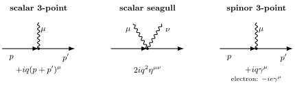
Minimal coupling produces different elementary vertices for scalar and spinor matter. Scalar QED has both the one-photon vertex and the seagull vertex . Spinor QED has the current vertex , which becomes for an electron of charge .
Spinor QED and the current vertex
Section titled “Spinor QED and the current vertex”For a Dirac field, the gauge-invariant Lagrangian is
For a field of charge ,
so
Thus
For the electron, , so
The difference between scalar QED and spinor QED is worth pausing over. The scalar kinetic term is quadratic in derivatives, so replacing by produces both and interactions. The Dirac kinetic term is first order, so minimal coupling produces only one power of . There is no elementary two-photon–two-fermion seagull vertex in ordinary spinor QED.
The charge-weighted coefficient of in the interaction is
Thus . For the electron, , consistently giving the vertex . With the previous page’s Maxwell-source convention , the source in is instead . This last minus sign is a dictionary between two named conventions, not an additional vertex sign.
Tree-level QED rulebook
Section titled “Tree-level QED rulebook”It is useful to fix what a diagram means before assembling amplitudes. We define by
Thus the product of propagators, vertices, and external wavefunctions supplied by a connected diagram is . The free internal-line factors are
For physical incoming and outgoing momenta and along a matter line, the vertices are
In an all-incoming convention, if labels the leg and labels the leg, the scalar three-point rule is . Since an outgoing scalar of momentum is represented by an incoming momentum , this is the same rule as . Incoming photons carry and outgoing photons carry ; the complex conjugation is not optional for circular polarization.
External wavefunctions and the one-photon current
Section titled “External wavefunctions and the one-photon current”At tree level, external fields are replaced by on-shell wavefunctions. For a fermion of momentum and spin ,
For a photon of momentum and polarization ,
The last relation says that the representative of the polarization vector is gauge-dependent. A physical amplitude must be unchanged by replacing by .
The elementary electron current couples to a photon line through
as a contribution to the diagram value . The current itself is well defined for momentum transfer that need not be lightlike, as in the virtual-photon exchange below. Its Ward check is immediate:
Using the Dirac equation on the left and on the right,
so
This is the simplest form of current conservation on an external line. It is also the tree-level seed of the Ward–Takahashi identities. It does not describe an allowed isolated emission or absorption of a nonzero real photon by a stable massive electron in empty space. For absorption, with future-directed and nonzero future-directed null would give
since in the electron rest frame . Emission has the same obstruction with and interchanged. The three-point current therefore serves here as a virtual-photon matrix element or an algebraic Ward check. Physical Compton scattering has two photons and the sum of two diagrams, as developed in the canonical tree-level QED calculation.
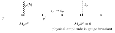
The on-shell electron-current Ward check, with equal electron masses and . Replacing by gives zero by the two Dirac equations. The diagram is schematic; it does not imply that an isolated electron can absorb or emit a nonzero real photon. In a physical process the appropriate full current or sum of diagrams must satisfy the Ward identity.
Photon exchange between charged particles
Section titled “Photon exchange between charged particles”The simplest nontrivial QED amplitude is one-photon exchange. For two distinguishable charged fermions with electron-like vertex , the tree contribution is
Equivalently,
for the stated -matrix and vertex conventions. More generally the numerator carries the product of the two charges, . The current–propagator–current structure is
In a covariant gauge, the extra propagator numerator is proportional to . It drops out because the on-shell currents obey . This both checks the momentum assignments and proves that the exchange amplitude is independent of the gauge parameter.
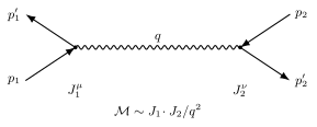
Tree-level photon exchange has the universal structure current–propagator–current. In Feynman gauge the internal photon contributes , while each fermion current contributes a spinor bilinear .
The nonrelativistic limit recovers the Coulomb interaction. Use a common orthonormal spin basis with two-component spinors . The leading temporal current is , so it preserves spin. For a slowly moving fermion with the same initial and final spin,
The momentum transfer has , hence
Therefore the dominant exchange is the temporal current coupled through
More explicitly, for charges and and spin preserved on each fermion line,
The relativistic Born-amplitude relation then gives
Fourier transformation yields the Coulomb potential,
This leading potential acts as the identity in the two fermions’ spin spaces. Spin-dependent interactions enter beyond this leading nonrelativistic approximation.
This is a useful sanity check: the same minimal coupling that enforces local gauge invariance also reproduces the familiar long-range electromagnetic force.
Scalar Compton scattering and the seagull term
Section titled “Scalar Compton scattering and the seagull term”Consider scalar Compton scattering,
The scalar QED Lagrangian produces three tree diagrams: two exchange diagrams and one contact diagram. The contact diagram is required by gauge invariance.
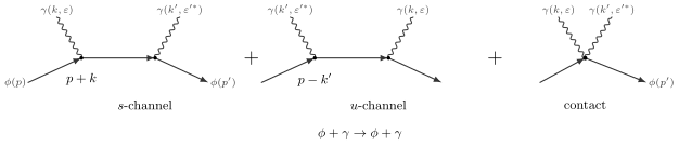
Scalar Compton scattering contains two scalar-exchange diagrams plus the contact interaction. The three diagrams are not separately gauge invariant; their sum is.
The three contributions have the schematic form
and
The precise placement of signs depends on whether all momenta are drawn incoming or as physical incoming/outgoing momenta. A reliable way to avoid confusion is to keep the scalar charge flow fixed along the line and then translate to the chosen all-incoming convention only at the end. What does not depend on notation is the Ward identity:
The cancellation works because, on shell,
and similarly for the other scalar-exchange channel. Thus the numerator of an exchange diagram can cancel its scalar propagator. The leftover local terms are canceled by the contact diagram. This is the practical reason why the term cannot be ignored even when one is mainly interested in one-photon vertices.
Spinor Compton scattering
Section titled “Spinor Compton scattering”For spinor QED,
there are two tree diagrams. There is no seagull vertex because the Dirac Lagrangian is first order in derivatives. With the electron-like vertex , the amplitude is
Here
The two terms are the two possible orderings of photon absorption and emission along the fermion line. Their matrix order matters because gamma matrices do not commute.
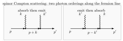
Spinor Compton scattering contains the two possible orderings of photon insertions along the fermion line. Gauge invariance belongs to the sum of the two diagrams, not to either diagram separately.
The Ward identity again comes from differences of inverse propagators. Strip off the common couplings and factors of , and write
where
on the nonsingular internal momenta. Contract the incoming-photon index with . In the first ordering use
The second term annihilates , while the first cancels and leaves . For the other ordering, momentum conservation gives
The first term annihilates and the second cancels the internal propagator with the opposite sign. Consequently,
This telescoping cancellation is the fermionic counterpart of the scalar-QED cancellation among exchange and contact diagrams. Repeating the argument with proves the Ward identity for the outgoing photon.
Spin sums and traces
Section titled “Spin sums and traces”After writing an amplitude, one often squares it and sums or averages over unobserved spin states. With the standard relativistic normalization,
The basic trace identities are
and
For example, a spin-summed fermion current product becomes
Evaluating the trace gives
A sum and an average are different operations. For an unpolarized process, sum over every unobserved final spin or helicity and divide by the number of equally populated initial states:
where for a massive particle and for a photon. For one-photon exchange between two incoming spin-one-half particles, the average factor is . Writing the charges as and the momentum transfer as , one obtains the useful trace form
where each averaged current tensor contains its own factor of ,
This separation is a useful defense against a common factor-of-two error: completeness relations perform sums, whereas the prefactor performs the initial-state average.
For photons, polarization sums must be handled with care. In a gauge-invariant amplitude, gauge-dependent pieces proportional to do not contribute, so one may effectively use
inside a complete gauge-invariant squared amplitude. The arrow is deliberate: the equality is not an identity of physical polarization vectors in an arbitrary gauge; it is a shortcut justified by Ward identities. A good practical test is this: before replacing a physical-polarization sum by , verify that the rest of the amplitude vanishes when any external polarization is replaced by its momentum.
Crossing as external-leg bookkeeping
Section titled “Crossing as external-leg bookkeeping”A time-ordered Green function does not know in advance which external legs will be interpreted as incoming particles, outgoing particles, incoming antiparticles, or outgoing antiparticles. These interpretations are imposed by LSZ reduction and by the choice of which pole is approached. Moving a charged external leg from one side of a process to the other turns it into an antiparticle and reverses the sign of the momentum in the analytic amplitude.
Schematically,
with the spinor wavefunction changed from a spinor to a spinor, or conversely, depending on the direction of the fermion arrow.
The external-wavefunction dictionary is
Thus crossing an outgoing antifermion replaces the analytically continued by an incoming-fermion assignment. For processes with several fermions, one must also preserve a fixed ordering of external fermionic operators. Reordering that convention can produce a relative minus sign; it is not captured by the shorthand alone.
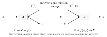
Crossing is the analytic continuation that moves an external leg across the amplitude. Momentum changes sign, and a particle becomes the corresponding antiparticle. Fermion arrows help keep the spinor factors in the correct order.
This is why Feynman rules are usually formulated with all momenta incoming and with continuous fermion-number arrows. Once the momentum and fermion ordering are fixed, the same analytic function describes several physical channels.
Summary
Section titled “Summary”Minimal coupling converts a global phase symmetry into a local gauge symmetry by replacing ordinary derivatives with covariant derivatives. For a complex scalar, this produces both a one-photon vertex and a two-photon seagull vertex. For a Dirac field, the first-order kinetic term produces the current interaction and hence the familiar photon–fermion vertex.
Tree amplitudes are assembled from external wavefunctions, propagators, vertices, and momentum conservation. Their most important consistency test is gauge invariance: replacing an external photon polarization by its momentum must give zero. For a single on-shell fermion current this follows directly from the Dirac equation. For scalar Compton scattering it follows only after the exchange diagrams and the seagull diagram are added together.
Spin sums turn squared amplitudes into traces of gamma matrices. Crossing then explains why the same analytic expression can describe several reactions: moving a charged external leg across the amplitude changes a particle into an antiparticle and sends . These are the practical tools needed before one-loop QED and power counting enter the course.
Common pitfalls
Section titled “Common pitfalls”Omitting the scalar seagull. The vertex is required by minimal coupling. Exchange graphs alone do not satisfy the two-photon Ward identities.
Testing gauge invariance diagram by diagram. A single exchange graph need not be gauge invariant. Apply the polarization-to-momentum replacement to the complete set of diagrams at the chosen perturbative order.
Using too early. This replacement is justified only inside a gauge-invariant squared amplitude. Gauge-dependent terms vanish after contraction with conserved currents or after the Ward-related diagrams have been summed.
Confusing sums with averages. Completeness relations sum over spin states; they do not divide by the number of initial states. Insert the initial-state average only once, after the amplitude has been squared.
Mixing charge signs with momentum-flow signs. The convention gives a fermion vertex ; for this is . The all-incoming convention changes the scalar momentum labels, not the underlying Ward identity.
Treating crossing as only . A crossed fermion also changes between and wavefunctions, and a fixed ordering of external fermions must be maintained. Any relative Fermi sign comes from that ordering, not from an arbitrary sign attached to crossing.
Exercises
Section titled “Exercises”Exercise 1
Section titled “Exercise 1”Derive the scalar QED three-point and four-point vertices from
Use the convention that the scalar enters with momentum and leaves with momentum .
Solution
Expanding the covariant derivative gives
Thus
The term linear in gives the one-photon vertex. With the standard scalar-line momentum assignment, the two derivative terms combine into . Including the factor of from , the vertex is
The quadratic term gives a vertex with two photon fields. Differentiating twice with respect to and gives a factor , and the factor of from gives
Exercise 2
Section titled “Exercise 2”Show that the on-shell fermion current
obeys
Solution
Let . Then
The Dirac equations are
Therefore
Substituting,
This is the tree-level Ward identity for a photon attached to an external on-shell fermion line.
Exercise 3
Section titled “Exercise 3”Using the trace identities in the text, prove that
Solution
Expand the trace:
because the terms with three gamma matrices have zero trace. Now use
and
Therefore
and the mass term adds . Combining terms gives
Exercise 4
Section titled “Exercise 4”In scalar QED, explain why the seagull graph is required for gauge invariance of scalar Compton scattering. You do not need to compute the full amplitude; show how replacing one polarization vector by its momentum cancels a scalar propagator.
Solution
Consider the part of the -channel diagram where the incoming photon of momentum attaches to an incoming on-shell scalar of momentum . The vertex contains
Replace by . Then
Since the external photon is on shell, , and since the scalar is on shell, . Hence
This is the inverse of the scalar propagator in that channel. Thus the Ward variation of the exchange diagram collapses the internal scalar propagator and leaves a local term. The corresponding variation of the other exchange diagram leaves another local term. These local remnants are canceled by the variation of the contact diagram from
Therefore the exchange diagrams alone are not gauge invariant; the complete minimal-coupling set is.
Exercise 5
Section titled “Exercise 5”Two distinguishable spin-one-half particles of charges scatter by one-photon exchange. Starting from
write the unpolarized squared amplitude as a product of two traces. Identify the initial-state average.
Solution
There are two spin states for each incoming particle, so the initial-state average is . Summing final spins and using the completeness relations gives
Equivalently, absorb one factor of into each current tensor. These averaging factors describe the unpolarized initial ensemble. Unobserved final spins are summed; a spin-selective measurement restricts or weights that sum according to the detector.
Further reading
Section titled “Further reading”- Coleman, Sidney. Lectures of Sidney Coleman on Quantum Field Theory. Edited by Bryan Gin-ge Chen, David Derbes, David Griffiths, Brian Hill, Richard Sohn, and Yuan-Sen Ting. World Scientific, 2019. DOI.
- Schwartz, Matthew D. Quantum Field Theory and the Standard Model. Cambridge University Press, 2014. DOI.
- Srednicki, Mark. Quantum Field Theory. Cambridge University Press, 2007. DOI.
- Weinberg, Steven. The Quantum Theory of Fields, Volume I: Foundations. Cambridge University Press, 1995. DOI.
- Zee, A. Quantum Field Theory in a Nutshell. 2nd ed. Princeton University Press, 2010. Publisher.