

Bogoliubov Coefficients and Pair Creation
The previous page separated two real-time questions. The in–out formalism computes transition amplitudes between a specified past vacuum and a specified future vacuum. The in–in formalism computes expectation values in the state actually prepared in the past. This page makes that distinction concrete by following a system whose Hamiltonian changes with time.
The model is deliberately simple: a harmonic oscillator whose frequency changes with time. In field theory, every momentum mode of a free field in a spatially uniform time-dependent background is such an oscillator. If the background changes, a mode that was positive-frequency in the past need not remain purely positive-frequency in the future. The coefficient of the negative-frequency component is the Bogoliubov coefficient . Its absolute square is the number of produced quanta in that mode.
This is the mechanism behind particle production in external fields, cosmological particle creation, parametric amplification, and the mode mixing that later appears near horizons. When the Hamiltonian is stationary in the remote past and future, the two asymptotic particle bases have an operational meaning and the comparison is sharp:
The particle concept remains basis-dependent, but the asymptotic mismatch is measurable: prepare the past vacuum and count quanta with detectors calibrated to the future Hamiltonian.
Required background. In–out and in–in functionals supplies the boundary-condition distinction used throughout, while free scalar mode quantization supplies the normalized oscillator expansion.
Helpful background. WKB, eikonal approximation, and turning points reviews complex turning points, and vacuum decay explains why an imaginary in–out effective action measures loss from the vacuum channel.
Time-dependent oscillator and conserved norm
Section titled “Time-dependent oscillator and conserved norm”Mode and correlator conventions. For the oscillator part of this page, positive frequency means . A normalized positive-frequency mode is
so that
The formulas below use and for annihilation operators associated with the past and future positive-frequency bases. Correlators are written without a leading , so the oscillator Feynman function obeys
Keeping this convention explicit prevents a common factor-of- error in the in–out Green function.
Consider a single real oscillator obeying
with asymptotically constant frequency,
A concrete example is
where is a finite disturbance. The equation is mathematically a one-dimensional scattering problem, except that the scattering coordinate is time. The conserved Wronskian is the analogue of flux conservation.
For any two solutions and , define the Klein–Gordon product
It is time independent. Indeed,
Choose the in-mode by its past behavior,
and choose the out-mode by its future behavior,
The pair is a basis of solutions. Therefore
The coefficients and are the Bogoliubov coefficients.
Taking the product with itself gives
while
Hence
This is not the ordinary conservation law of Schrödinger scattering. The negative-frequency solution has negative Klein–Gordon norm, so the group of transformations is hyperbolic rather than unitary. The same minus sign is responsible for amplification and pair creation.
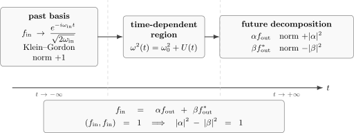
A positive-frequency in-mode passes through a time-dependent background and becomes a mixture of positive- and negative-frequency out-modes. Wronskian conservation gives .
Operators and particle number
Section titled “Operators and particle number”Quantize the oscillator by expanding the same Heisenberg operator in either basis:
Substitute
and compare coefficients of and . One obtains
The commutator is preserved precisely because
The in-vacuum and out-vacuum are defined by
The number of future quanta in the past vacuum is
This is the first central result:
The result is not obtained by saying that the vacuum “contains particles” in an absolute sense. It says something operational: prepare the state with no particles in the past, let the background act, and count particles using detectors calibrated to the future Hamiltonian.
The in-vacuum as a squeezed out-state
Section titled “The in-vacuum as a squeezed out-state”The relation between the two vacua is especially transparent. Invert the Bogoliubov transformation:
The in-vacuum obeys
Now use the identity
It follows that
The normalization is fixed by . Since
one finds
Thus the vacuum persistence probability for one real oscillator is
The exponential contains only even powers of . A centered time-dependent quadratic Hamiltonian preserves number parity and therefore creates quanta in pairs. Expanding the squeezed state gives
Since
the amplitude ratio is
Odd-particle amplitudes vanish in this simple quadratic problem. The probability distribution is
The probabilities sum to one because
The mean occupation number is
as it must be.
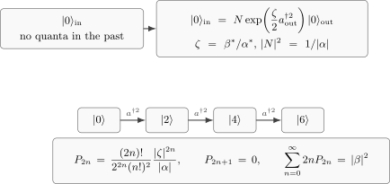
The past vacuum is a squeezed state in the future basis. For a single real oscillator, only even occupation numbers occur, and the distribution is controlled by .
In–out propagator and pair amplitudes
Section titled “In–out propagator and pair amplitudes”The ordinary Feynman Green function with in–out boundary conditions is
It is the inverse of the differential operator with Feynman boundary conditions: negative frequency toward the far past and positive frequency toward the far future. With the mode conventions above,
The factor is not decorative. It normalizes the derivative jump at so that
To see the pair amplitude inside the Green function, take both times late. Then
and therefore
For equal future frequency , this is
The first term is ordinary propagation in the out-vacuum. The second term has the time dependence of two future annihilation operators acting on the in-vacuum:
Comparing coefficients gives
which is the case of the squeezed-state result above.
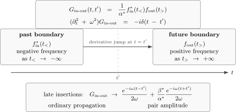
The in–out Green function is fixed by a negative-frequency condition in the past and a positive-frequency condition in the future. When both insertions are late, it contains both ordinary propagation and a pair-production amplitude.
This is why in–out correlators are excellent for extracting amplitudes. They are not, however, expectation values in the produced state. For actual particle number, current, energy density, or backreaction, one should use in–in quantities.
Field theory: one oscillator per momentum mode
Section titled “Field theory: one oscillator per momentum mode”For a real scalar field in a spatially uniform time-dependent background,
For literal number operators and normalized vacuum vectors, first use a periodic box of spatial volume and a finite, inversion-symmetric momentum cutoff. Each retained oscillator must have positive asymptotic frequency; a massless zero mode needs separate treatment. Box operators obey and multiply normalized spatial waves . The corresponding continuum Fourier notation is
with
It is safest to include the spatial plane wave in the mode label. With
complex conjugation reverses momentum, and the normalized modes satisfy
Consequently,
and momentum conservation makes quanta appear in opposite-momentum pairs. For an isotropic background, and . In the regulated box, the normalized squeezed state has the form
with an overall normalization given by the finite product over independent modes. The future occupation in one normalized box mode is
The factor in the exponent compensates for summing over both and . One may instead sum over one representative of each distinct pair and omit that factor. A self-paired zero mode retains the single-oscillator factor.
In continuum normalization, , and the distributional statement is
Thus is an occupation per normalized mode, while the total number and its thermodynamic density are
when the ultraviolet and infrared limits converge. Setting the continuum delta function to one would lose the volume factor.
Removing the mode cutoff at fixed volume requires for a bounded canonical map to be unitarily implementable. Finite density in infinite volume is a different statement: a nonzero homogeneous continuum mixing need not define a vacuum vector in the original Fock space. Bogoliubov transformations and unitary implementability explains this distinction and the precise Hilbert–Schmidt test. The squeezed vector and vacuum product here are regulated statements, not an assumed global unitary in the thermodynamic limit.
The vacuum persistence probability is a product over modes. Equivalently,
where is the in–out effective action. A nonzero imaginary part of is therefore the many-mode version of the statement : the vacuum-to-vacuum channel has lost probability to states with particles.
For bookkeeping, distinguish two related squeeze problems. One real oscillator has
whereas one independent particle–antiparticle or two-mode pair has
The momentum product must count independent pairs only; any self-paired real zero mode is counted as one real oscillator. For a complex charged field and nonzero , the pair and the pair are distinct. At zero momentum, and still form a two-species pair. Thus all particle momenta label independent particle–antiparticle pairs. The volume factor and the distinction between mean multiplicity and vacuum survival are explicit in Gelis and Tanji 2015, §3.3, Eqs. (71)–(75), PDF pp. 22–23. In particular, a vanishing infinite-volume vacuum overlap does not by itself imply a divergent particle density.
Perturbative and adiabatic estimates
Section titled “Perturbative and adiabatic estimates”The coefficient is a reflection amplitude in time. If
then the first Born approximation gives
The phase is the energy cost of producing two oscillator quanta. Slow backgrounds have little Fourier support at frequency , so production is small.
A more geometric estimate comes from WKB. Write
where the adiabaticity parameter is
If on the real axis and is analytic, pair production is controlled by complex turning points where
for a real analytic profile. When a single conjugate pair dominates, the probability has the schematic form
The contour, Stokes sector, and possible interference among several turning-point pairs are part of the approximation; the displayed formula records only the leading isolated-pair exponent. It makes precise the old intuition that a particle can be created only by a sufficiently nonadiabatic background. If the background changes abruptly, is often only power-law suppressed. In the analytic, slowly varying regime with the isolated turning points specified above, production is exponentially suppressed.
A useful special case is a very slow change of mass. If the frequency evolves from to over a time scale with , the action variable of the oscillator is adiabatically conserved and . The energy changes because the Hamiltonian changes, but the occupation number does not.
Pair creation in a spatially uniform electric field
Section titled “Pair creation in a spatially uniform electric field”Now consider a charged scalar field in a classical electric field pointing in the direction. Use the gauge
Here denotes the -component of the spatial vector . With the mostly-minus metric, the covariant four-potential is . Thus gives the kinetic momentum .
Here is the signed coefficient in the covariant derivative. The positive-frequency particle sector has Maxwell-source charge : with the inherited action convention, the current obtained by varying the matter action is the negative of the source in . The current derivation below fixes this sign explicitly. Thus , and a positive source charge accelerates along the electric field. The scalar action and derivative convention agree with Gelis and Tanji 2015, §3.1, Eq. (54), PDF pp. 18–19, with their ; positive-charge acceleration must still be assigned to the stated particle sector.
For derivative coefficient , a Fourier mode
obeys
This is again a time-dependent oscillator. The canonical momentum labels the Fourier mode. The physical kinetic momentum is
For a constant electric field, choose
Then
The mode is most nonadiabatic near the time when the kinetic longitudinal momentum crosses zero,
The complex turning points are
The WKB exponent is
Therefore
for a constant field. This is the exact mean occupation number per scalar mode in an eternal uniform field, and it is also the locally constant result for a long pulse away from its switching regions. Because an eternal field never becomes field-free, its in/out states are defined by the positive-frequency WKB branches as , not by free plane waves with a fixed kinetic momentum.
The mode exponent also gives the leading pair-production rate in a long constant field. During a time interval in a box of length , the kinetic momentum sweeps through the nonadiabatic region for
longitudinal modes. Therefore, in dimensions and in the dilute scalar limit, the mean number of produced pairs satisfies
This is the leading term in the scalar Schwinger rate. The full vacuum persistence probability resums multiple production events and, for spinor QED, includes spin degeneracy and Fermi statistics.
In the figure, distinguish the mode label from the physical source charges on the separating particles. The upper panel shows the minimum real gap; the lower panel shows which charge accelerates in each direction.
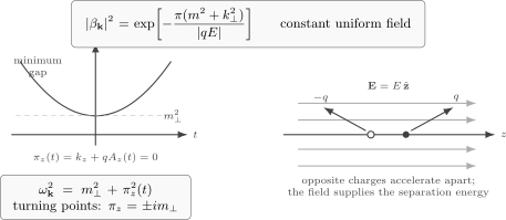
A spatially uniform electric field gives , with . The minimum real gap and adjacent complex turning points fix the constant-field production exponent. For the illustrated and , the particle has source charge and accelerates left, while its antiparticle accelerates right. The geometry is schematic, with no numerical axis scale; the displayed constant-field exponent is exact for the prescribed scalar background.
There is also a simple spacetime estimate behind the exponent. To create a pair of rest mass , the field must do work of order . If the particles separate by a distance , the work is roughly
Quantum mechanics allows such a process through tunneling over a distance of order
The precise calculation replaces this estimate by the exponential , but the physical content is the same: strong fields shorten the tunneling distance and enhance pair production.
In–in current and backreaction
Section titled “In–in current and backreaction”The in–out effective action tells us whether the vacuum remains the vacuum. The electric current produced by the pairs is an in–in observable. For , variation with respect to the covariant potential gives
With the Maxwell term , its equation and the physical source current are
These signs also fix the particle charge. For a unit-normalized positive-frequency plane wave, the action-current charge is , so the Maxwell-source charge is . Its antiparticle has charge . A spatial lower index introduces an additional minus sign: and .
To fix the mode normalization, expand the complex field in a spatially homogeneous background as
Both time functions solve the same real oscillator equation for this Fourier label, and . The and operators have the continuum commutator given above and annihilate the in-vacuum. Since on each spatial plane wave, the vacuum contraction in the sector gives
The subscript denotes subtraction of the local ultraviolet terms with a consistent gauge-invariant current prescription, including charge renormalization, for example the appropriate adiabatic subtraction. It does not mean that arbitrary mode-by-mode vacuum removal is gauge invariant. One may first derive the contractions with regulated sums; a fixed canonical-momentum cutoff alone is not the final gauge-invariant prescription.
After a pulse has ended, let be the constant future frequency and write . Subtracting the out-vacuum term leaves
If the oscillatory coherence dephases under momentum integration or an explicitly coarse time resolution, the conduction part is
The factor two counts the two charges in each pair: and have the same sign. The full transient current also contains coherence and vacuum polarization; it is not determined by particle number alone or by the instantaneous value of .
For an electric-field pulse, the vector potential changes by
Thus the signed kinetic-momentum change is
and a late-time current can depend on this accumulated impulse. This is not a violation of gauge invariance. A constant shift of is compensated by relabeling the canonical momentum , while the difference is fixed by the physical field history.
The next figure isolates a possible late conduction current after a positive pulse. Its curves illustrate retained production and impulse, not a computed transient current or a claim that coherence always decays monotonically.
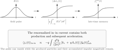
Schematic collisionless response for and a positive pulse: the particle’s signed impulse is , while its source charge is . The particle and antiparticle contributions to can therefore add to a positive conduction current after the pulse. The late curve assumes produced pairs and dephased coherence; it is not a numerical solution for the full renormalized transient current. All curves have arbitrary vertical scales.
If the electric field is externally prescribed, this current is an output. For a homogeneous dynamical field, Maxwell’s equation is in the normalization above. A positive conduction current drains a positive field; energy balance gives . Continuous production eventually invalidates the fixed-background approximation. Coherent transients and plasma oscillations can occur, so screening need not be monotonic.
Periodic driving and moving-frame instabilities
Section titled “Periodic driving and moving-frame instabilities”Next contrast nonperturbative production with ordinary thresholds. Suppose a weak perturbation contains a Fourier component of frequency . At first order, creating two massive quanta requires
At th order, quanta of the drive can combine, and the threshold becomes
At any fixed perturbative order, sufficiently small lies below that order’s threshold. This does not forbid a strong slowly varying field from creating pairs through complex turning points. At nonzero , sufficiently high multiphoton orders can also cross the threshold. The constant-field Schwinger factor is the distinct zero-frequency example: it is nonanalytic in the field strength at and therefore invisible at every finite order in a power series in .
The same energy-accounting logic diagnoses a moving body’s energetic instability. Suppose a heavy impurity moves at through a homogeneous medium at zero temperature. For a branch with at nonzero momentum, the leading net energy cost of transferring momentum from the body into one excitation is
The neglected nonrelativistic recoil term is for impurity mass . In the infinite-mass limit, a negative-cost excitation exists precisely when
The denominator must retain the direction of motion when the dispersion is anisotropic Yu 2017, Eqs. (1)–(3), PDF p. 1. For an isotropic branch , choosing momentum parallel to the velocity minimizes the cost at fixed , and this reduces to . A minimum may fail to be attained; equality does not give a negative-cost excitation.
For example, gives for motion along , since . Minimizing instead gives 1 along , where the body transfers no energy. For the isotropic linear branch , the criterion is .
This is an energetic threshold for the specified branch and heavy-impurity problem. An actual emission rate also requires an allowed coupling, nonzero matrix elements, and energy-conserving phase space. Other excitation channels can set a lower threshold. It does not explain Rindler thermality: an accelerated observer in vacuum instead changes the time generator and has access to only one causal wedge.
In a compact isolated system, a permanently driven state need not approach a steady state. Energy has nowhere to escape, recurrences can matter, and backreaction must eventually be included.
Summary
Section titled “Summary”A time-dependent quadratic background mixes positive and negative frequencies. The phase of the Bogoliubov coefficient depends on mode conventions, while measures the mixing invariantly and is the number of produced quanta in the corresponding out-mode. The identity
is Wronskian conservation, or equivalently preservation of canonical commutation relations.
The in-vacuum is a squeezed state in the out-basis. For a single real oscillator,
In–out propagators contain transition amplitudes such as . In–in expectation values contain actual observables such as produced particle number, current, energy density, and backreaction.
A spatially uniform electric field turns each charged momentum mode into a time-dependent oscillator with
For a constant field,
which is the basic Schwinger exponent. The next page will use the same positive/negative-frequency logic in a different setting: mode functions adapted to accelerated observers and Rindler wedges.
Common pitfalls
Section titled “Common pitfalls”The most common mistake is to call a reflection coefficient and then impose . That is the wrong conservation law. Negative-frequency modes have negative Klein–Gordon norm, so the correct identity is .
Another common mistake is to treat particle number as absolute. In time-dependent backgrounds, particle number is defined with respect to a choice of positive-frequency modes. It is unambiguous when the background becomes time independent in the past and future. If the background never switches off, one must use an adiabatic, detector-based, or otherwise physical prescription.
Finally, an in–out current is not the produced current. The in–out effective action diagnoses vacuum persistence and transition amplitudes. Backreaction is driven by the in–in Maxwell-source current . Do not identify a spatial lower component with the upper component, or the derivative coefficient with the source charge of the chosen positive-frequency mode.
A further trap is to identify every exponentially small production process with a perturbative threshold. Multiphoton thresholds depend on Fourier support and order in the driving amplitude; the Schwinger process is nonanalytic at and is controlled by complex turning points.
Exercises
Section titled “Exercises”Exercise 1: Wronskian normalization
Section titled “Exercise 1: Wronskian normalization”Let and assume
Show that implies .
Solution
Use sesquilinearity of the Klein–Gordon product:
The cross terms vanish because
Thus
Since is normalized to one,
Exercise 2: squeezed-state probabilities
Section titled “Exercise 2: squeezed-state probabilities”Starting from
derive the squeezed-state expression for and the probability
Solution
The condition becomes
Try
Since
the vacuum condition gives
Expanding the exponential,
Using
we get
The normalization is
Because
we find
Therefore
Exercise 3: Born approximation for mode mixing
Section titled “Exercise 3: Born approximation for mode mixing”For
show that the first Born approximation has the form
up to a convention-dependent overall phase.
Solution
Write the solution as a slowly corrected superposition of free modes,
with and . To first order in , one may compute the negative-frequency amplitude generated by the perturbation using the free retarded Green function of :
The equation is
Insert the zeroth-order solution
on the right-hand side. The late-time correction is
For later than the support of ,
The coefficient of is therefore
Changing the phase convention for the negative-frequency mode changes the overall phase of , but not .
Exercise 4: constant-field Schwinger exponent
Section titled “Exercise 4: constant-field Schwinger exponent”For a charged scalar in a constant electric field, use
and the complex turning points
to show that
Solution
The answer depends only on , so take while evaluating the oriented contour; reversing the field interchanges the two turning points. The WKB exponent is
Set
The turning points become
Thus
Put , with running from to . Then and
Therefore
The remaining integral is the area of a semicircle of radius :
Hence
The tunneling probability is the exponential of minus this quantity:
Exercise 5: produced occupation number
Section titled “Exercise 5: produced occupation number”Show directly from
that the in-vacuum contains out-quanta on average.
Solution
Compute
Using
we get
where . Expanding,
Taking the expectation value in the in-vacuum kills all terms except the last one:
Therefore
Exercise 6: dilute scalar production rate
Section titled “Exercise 6: dilute scalar production rate”Use the mode probability
for a constant electric field in dimensions to derive the dilute scalar estimate
Solution
In a time , the longitudinal kinetic momentum changes by
With box normalization, the density of longitudinal modes is , so the number of longitudinal modes that pass through the nonadiabatic region is
The number of produced pairs is therefore
Divide by and by :
The Gaussian integral is
Thus
This calculation gives the leading dilute production rate, not the full multi-pair vacuum persistence formula.
Exercise 7: Landau critical velocity
Section titled “Exercise 7: Landau critical velocity”An excitation branch has for nonzero momentum in the medium rest frame. In the infinite-mass impurity limit, show that a negative-cost excitation exists for motion along precisely when
Recover the isotropic result, and evaluate the threshold for with motion along . Explain why this criterion alone does not determine an emission rate.
Solution
In the heavy-body limit, transferring momentum changes the body’s kinetic energy by to leading order. The net energy cost is therefore
If , the cost is positive. Otherwise, dividing by the positive longitudinal projection gives
Some momentum satisfies this inequality precisely when exceeds the infimum. At equality no ratio lies below . If depends only on , alignment with maximizes the denominator without changing the numerator, giving
For a linear isotropic branch , this is . For the anisotropic example, gives , with equality at , so . The unrelated radial minimum 1 lies along and cannot describe motion along . A nonzero rate further requires a coupling to the mode and energy-conserving phase space; a forbidden matrix element is not repaired by a negative energy cost.
References
Section titled “References”- Gelis, François, and Naoto Tanji. “Schwinger Mechanism Revisited.” Progress in Particle and Nuclear Physics 87 (2016): 1–49. DOI; Open PDF, 2015 preprint v1.
- Yu, Zeng-Qiang. “Landau Criterion for an Anisotropic Bose–Einstein Condensate.” Physical Review A 95 (2017): 033618. DOI; Open PDF, preprint v1.
Further reading
Section titled “Further reading”- Birrell, N. D., and P. C. W. Davies. Quantum Fields in Curved Space. Cambridge Monographs on Mathematical Physics. Cambridge University Press, 1982.
- Dunne, Gerald V. “Heisenberg–Euler Effective Lagrangians: Basics and Extensions.” In From Fields to Strings: Circumnavigating Theoretical Physics, edited by M. Shifman, A. Vainshtein, and J. Wheater, vol. 1, 445–522. World Scientific, 2005.
- Kim, Sang Pyo, and Don N. Page. “Schwinger Pair Production in Electric and Magnetic Fields.” Physical Review D 73 (2006): 065020.
- Parker, Leonard, and David Toms. Quantum Field Theory in Curved Spacetime: Quantized Fields and Gravity. Cambridge University Press, 2009.
- Schwartz, Matthew D. Quantum Field Theory and the Standard Model. Cambridge University Press, 2014, chapters 33–34.
- Schwinger, Julian. “On Gauge Invariance and Vacuum Polarization.” Physical Review 82 (1951): 664–679.
- Weinberg, Steven. The Quantum Theory of Fields. Vol. 1, Foundations. Cambridge University Press, 1995.