

Mass Tuning and Relevant Deformations
The previous page used the running quartic coupling and the running normalization of the thermal operator to derive the logarithmic specific-heat singularity at the four-dimensional upper critical dimension. That calculation had a quiet but essential assumption: the theory was close enough to criticality that the RG flow could run for many decades before being stopped by a physical mass.
This page makes that assumption explicit. A scalar theory near a continuous transition has at least one relevant parameter: the coefficient of . This parameter is not just another coupling. It decides whether the infrared theory is critical or massive. If it is tuned to a special value, the correlation length diverges and the logarithmic critical behavior of the previous page is visible. If it is not tuned, the flow stops at the inverse correlation length, and the long-distance theory becomes insensitive to further critical running.
The main lessons are:
and criticality is the condition
which usually requires an additive tuning of the bare quadratic coefficient.
Helpful background. Källén–Lehmann representation distinguishes a lightest spectral mass from a small-momentum expansion of the propagator. Critical exponents and hyperscaling explains the correlation-length scaling used below and the role of dangerously irrelevant couplings.
Relevant directions and the critical surface
Section titled “Relevant directions and the critical surface”Cutoff action and stopping scale
Section titled “Cutoff action and stopping scale”We use a cutoff scalar theory in four Euclidean dimensions,
where is the bare quadratic coefficient. We work in the -symmetric sector, with no external field linear in , and in the basin of the ordinary continuous transition with positive quartic coupling. The mass-scaling calculation approaches that transition from the symmetric phase. The symbol is useful because in statistical mechanics it is proportional, after an additive shift, to the reduced temperature. In particle-physics notation one often writes .
For the one-component theory,
and the leading-log normalization of a insertion is
Let denote the exponential correlation length of the connected order-parameter two-point function. Its inverse defines the infrared mass used here,
Thus is the scale where the critical RG flow stops. If an isolated lightest pole with nonzero overlap controls this correlator, is its pole mass; more generally the lightest spectral threshold controls the exponential decay.
At the Gaussian fixed point in Euclidean dimensions, a scalar field has engineering dimension
Therefore
The action is dimensionless, so the coupling multiplying a local operator has engineering dimension . In ,
Thus the mass term is relevant, the quartic coupling is marginal by power counting, and a term is irrelevant. Written in terms of dimensionless couplings at scale ,
coarse graining toward the infrared gives, at tree level,
The relevant variable grows as the theory is viewed at longer distances. The irrelevant variable shrinks. The quartic coupling is special in four dimensions: it is marginal at tree level, and loop effects make it run only logarithmically.
The relevant mass direction is why a critical point is not generic. Within this -symmetric sector and ordinary critical basin, the condition defines a surface of codimension one. A symmetry-breaking external field would supply another relevant direction and would also have to be tuned. Moving along the symmetric critical surface changes marginal and irrelevant couplings while preserving criticality; moving away produces a finite correlation length.
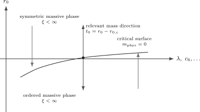
The critical surface in the -symmetric sector is the set of bare actions whose correlation length diverges. The deviation is a relevant coordinate: it grows under coarse graining and sends the theory into a phase with finite connected correlation length. The drawing is schematic.
The critical value is not generally . It is a function of the cutoff and of the other bare couplings,
The scaling variable is the deviation from this surface,
In a magnetic system, is proportional to after a nonuniversal normalization. In a relativistic scalar theory, is the renormalized mass-squared parameter, again up to multiplicative logarithmic factors.
The physical mass stops the flow
Section titled “The physical mass stops the flow”At the critical point, there is no intrinsic infrared scale. If we compute a vertex at external momentum , the logarithmic flow can run down to . Away from the critical point, the long-distance two-point function is massive,
in the single-pole, leading-log approximation just specified. The mass cuts off the critical singularities. For momenta , the field still behaves approximately as a critical field; for , the propagator no longer looks scale invariant.
A natural matching scale for the low-energy quartic interaction is . Write for the coupling matched there at leading-log accuracy in this scheme:
Relating it to a specified measured amplitude also requires field normalization and finite matching terms, which are beyond this approximation. A mass-independent subtraction scale may continue to run below ; it must not be identified there with the momentum dependence of a physical massive amplitude. For intermediate scales , the same running coupling can be expressed in terms of . Since
and
we subtract the two equations and obtain
Equivalently,
This formula is just the previous running coupling with a different boundary condition. Instead of specifying the bare coupling at the cutoff, we specify the physical coupling at the mass scale.
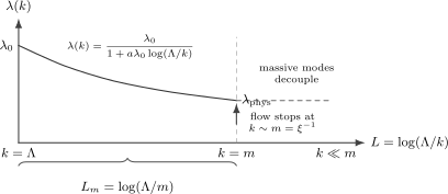
At leading-log accuracy the critical running stops at . The labeled is the matching value in the scheme defined above; the dashed plateau schematically represents massive low-energy response, not continued mass-independent subtraction-scale evolution.
There is an important consequence. If is fixed and the cutoff is taken far above the physical mass, then
At leading-log accuracy,
Thus the four-dimensional one-component theory approaches a free theory in this continuum limit. Conversely, if one insists on holding a positive finite fixed, then
For sufficiently large , the right-hand side becomes negative. Perturbatively this is the Landau-pole obstruction written backward: the theory is perfectly useful as an effective field theory with a finite cutoff, but the interacting continuum limit is not obtained by taking at fixed positive physical coupling.
Additive mass renormalization
Section titled “Additive mass renormalization”The mass term is relevant not only in the infrared. It is also the local operator most easily generated by ultraviolet loops. This is why the critical value depends on the cutoff.
In the symmetric massive theory, take for the following explicit cutoff integral. In the theory
the one-loop tadpole contributes a local self-energy
With a spherical Euclidean cutoff,
Thus, for ,
The quadratic term is specific to a cutoff description; a scaleless massless tadpole vanishes in dimensional regularization. The position of the critical surface and the split into a bare parameter and local corrections depend on that description. With the hard cutoff retained, higher loops generate further local terms of the schematic form
where the constants depend on the cutoff convention and on how the local part is separated from the nonlocal part.
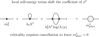
The bare quadratic term and zero-momentum self-energy determine , shown schematically with cutoff-dependent coefficients suppressed. Its vanishing locates the ordinary critical point from the symmetric phase. Away from criticality, the second-moment mass also needs the slope , while an exact pole mass requires the momentum-dependent inverse propagator.
The zero-momentum tuning condition is therefore expressed by
Here includes the regulated self-energy and the chosen counterterms. At one-loop tadpole order it is momentum independent, so the pole and curvature definitions agree to that order. Beyond it, an isolated pole instead solves , and . The critical bare value is the one for which vanishes:
After subtracting the critical value, the remaining deviation
is the relevant scaling field. In a statistical system this tuning is ordinary experimental control: changing moves the system through . In a fundamental scalar theory the same statement becomes the naturalness problem: a small physical scalar mass requires a cancellation between a bare parameter and cutoff-sensitive local quantum corrections.
Correlation length and logarithmic mass scaling
Section titled “Correlation length and logarithmic mass scaling”The previous page only needed the rough relation
inside a logarithm. That is enough for the specific-heat logarithm because constants and powers inside the logarithm change only subleading terms. But the mass itself also receives a logarithmic correction at the upper critical dimension.
Let
be the positive deviation from the critical surface on the symmetric side, . It has dimensions of mass squared. A mass perturbation inserts the thermal operator
At momenta still above the physical mass, the leading-log dressed insertion carries the factor
Thus the inverse propagator in the critical regime has the schematic form
The flow stops when the two terms become comparable at :
Therefore
Solving this relation asymptotically gives, up to nonuniversal constants inside the logarithm,
The mean-field exponent survives in four dimensions, but it is dressed by a universal power of a logarithm. The exponent is for the one-component scalar theory with the normalization used here. The logarithm has a dimensionless argument; its constant scale and the overall amplitudes are nonuniversal. For one must expand about the ordered minimum: already at tree level its curvature is , rather than . The symmetric-phase self-consistency equation is not a derivation of broken-phase amplitudes. For an model the logarithmic power and possible Goldstone infrared behavior require their own analysis.
This is the same physics as the logarithmic specific heat: the Gaussian fixed point controls the power law, while the marginally irrelevant quartic coupling controls the logarithmic correction.
A finite external momentum and a finite physical mass cut off the critical shells. In a box of size , the smallest nonzero momentum is of order . The nonzero-mode leading logarithm therefore stops at
One then replaces
for those shells. A periodic box also contains a constant mode; it has not been removed by . At criticality its quartic action, schematically , must still be integrated. This is why the replacement alone does not determine finite-size susceptibility or order-parameter fluctuations. Boundary conditions that remove the constant mode give a different finite-size problem.
Irrelevant operators and shifted critical data
Section titled “Irrelevant operators and shifted critical data”The effective action contains every local operator allowed by the symmetries. The reason this does not destroy predictivity is the scaling hierarchy. In four dimensions,
has a dimensionless coefficient at scale of order
It dies in the infrared near this fixed point. Such an operator can still affect local quantities. For example, contracting fields inside can shift the coefficient of , the coefficient of , and therefore the numerical value of . After retuning within the same ordinary critical basin, it does not change the leading logarithms governed by the marginal quartic coupling and the relevant thermal scaling field. This statement excludes tuning to a tricritical point or changing the couplings so that the transition becomes first order.
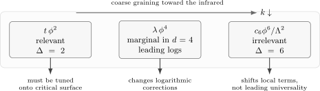
Near the ordinary four-dimensional scalar critical point, is relevant, is marginal with logarithmic running, and is irrelevant. Within this critical basin, irrelevant operators can shift the critical surface while preserving its leading logarithms. The classification is schematic and does not describe tricritical tuning.
This also explains why dimensions above four behave differently. Consider the massless bubble integral in dimensions,
For away from even dimensions, the nonlocal term after local ultraviolet subtractions has the power dependence
while local cutoff-dependent pieces are analytic in and are absorbed into local counterterms. At even , the corresponding term is proportional to , with a reference scale understood in the logarithm; d=4 gives the unsuppressed logarithm. For , the massless integral also needs infrared regulation even at nonzero external Euclidean momentum. In , the dominant term is cutoff dependent and local, schematically
with no large logarithm. The quartic coupling has engineering dimension and is irrelevant. The leading bulk critical powers are mean-field, and the four-dimensional logarithmic corrections are absent. The quartic coupling is nevertheless dangerously irrelevant above four dimensions: it is needed to stabilize the ordered phase and can enter amplitudes, finite-size scaling, and hyperscaling relations through inverse powers. “Irrelevant” describes its linearized flow near the Gaussian fixed point, not permission to delete it from every observable.
What has been separated
Section titled “What has been separated”It is useful to separate three kinds of statements that are often mixed together.
First, the critical surface is determined by local UV-sensitive data. The value depends on the regulator, the cutoff, and irrelevant couplings. This dependence is not universal.
Second, the scaling variable is the deviation from the critical surface,
This is the relevant parameter that determines the inverse correlation length.
Third, the universal long-distance behavior is determined by the RG flow near the fixed point. In four-dimensional theory, the quartic coupling is marginally irrelevant, so universal critical behavior contains logarithms rather than new non-mean-field powers.
This separation is the operational content of renormalization. UV fluctuations move the coordinates of the critical surface, while the RG flow near that surface controls universal long-distance singularities.
The next page turns this local viewpoint into an algebra of operators. Instead of asking only how couplings run, we ask what happens when two local fields approach one another. The answer is the operator product expansion.
Summary
Section titled “Summary”The coefficient of is relevant. In four dimensions,
so the dimensionless mass variable grows under coarse graining as the theory flows toward the infrared.
The condition for criticality is not , but
or equivalently
The deviation
is the relevant scaling variable.
A nonzero physical mass stops critical running at
The quartic matching value at that scale, to the stated leading-log accuracy, is
Equivalently,
Local self-energy corrections shift the mass additively. With a hard cutoff,
This shift determines the nonuniversal location of the critical surface.
On the symmetric side , the leading-log relation between the infrared mass and the thermal scaling variable is
so
Within the ordinary critical basin, irrelevant operators such as can shift and other local data while preserving the leading logarithms controlled by the marginally irrelevant quartic coupling.
Common pitfalls
Section titled “Common pitfalls”Do not identify the bare mass , the exponential mass , and the second-moment mass . The latter uses the value and slope of the inverse propagator at zero momentum; its equality with an isolated pole mass requires an approximation or a special spectral form.
Do not locate the critical point by setting the bare quadratic coefficient to zero. The correct condition is , and generally contains cutoff-dependent loop corrections.
Do not run critical logarithms below the mass scale. Once , the propagator is massive and the critical RG flow is cut off.
Do not treat the coefficient of a quadratic divergence as universal. A hard cutoff, a lattice cutoff, Pauli–Villars fields, and dimensional regularization organize local mass terms differently. The need to tune a relevant scalar mass is physical; the numerical coefficient of a cutoff-dependent local term is not universal.
Do not confuse irrelevant with nonexistent. Irrelevant operators affect the location of the critical surface and analytic background terms. They are irrelevant to leading infrared singularities, not irrelevant to every number in the microscopic theory.
Do not conclude from logarithmic triviality that the cutoff theory is useless. Four-dimensional theory is an excellent effective theory over a finite range of scales. The obstruction concerns the interacting continuum limit at fixed positive physical coupling.
Exercises
Section titled “Exercises”Exercise 1 — Gaussian operator classification
Section titled “Exercise 1 — Gaussian operator classification”At the Gaussian fixed point in Euclidean dimensions, show that
and find the engineering dimensions of the couplings multiplying , , and . Classify these operators in .
Solution
The kinetic term is
Since the action is dimensionless, and , we require
Therefore
For an operator ,
The coupling in
has dimension
Thus
In ,
Therefore is relevant, is marginal by engineering dimension, and is irrelevant.
Exercise 2 — The hard-cutoff tadpole
Section titled “Exercise 2 — The hard-cutoff tadpole”Evaluate the leading large- behavior of
Use it to find the one-loop tadpole mass shift in theory.
Solution
In four Euclidean dimensions,
Therefore
Set , so . Then
Since
we get
For ,
In theory, the one-loop tadpole self-energy has the combinatorial factor , so
Thus
The quadratic term is cutoff-scheme dependent and local. It is absorbed into the location of the critical surface.
Exercise 3 — Matching at the physical mass
Section titled “Exercise 3 — Matching at the physical mass”Let
and define
Show that
What happens to as with fixed positive ?
Solution
Invert the running coupling:
At ,
Subtract the second equation from the first:
Therefore
or
For fixed positive ,
As , the denominator grows without bound, so
This is the leading-log form of triviality for the continuum limit of positive four-dimensional theory.
Exercise 4 — The correlation-length logarithm
Section titled “Exercise 4 — The correlation-length logarithm”Assume the dressed thermal insertion is
and that the infrared mass obeys the leading-log single-pole relation on the symmetric side,
Derive the leading logarithmic behavior of the correlation length as , keeping the logarithm’s argument dimensionless.
Solution
The defining relation is
As , the mass becomes small, so the logarithm is large. To leading logarithmic accuracy, the mean-field relation gives inside the logarithm. Therefore
Thus
Taking the square root,
Since ,
The power is the mean-field exponent, while is the logarithmic correction exponent for the one-component theory.
Exercise 5 — How an irrelevant operator shifts critical data
Section titled “Exercise 5 — How an irrelevant operator shifts critical data”In four dimensions, consider the irrelevant perturbation
Show by power counting that its dimensionless strength at scale is of order . Within the ordinary critical basin specified above, explain why it can shift while preserving the leading critical logarithms.
Solution
In four dimensions,
The coupling multiplying must have dimension
Writing it as makes dimensionless at the cutoff scale. At a lower scale , the natural dimensionless strength is obtained by multiplying by :
Thus the perturbation becomes small in the infrared.
However, loops involving can contract fields at short distances and generate local lower-dimension operators, including and . These contributions shift nonuniversal quantities such as the critical value and hence . After the critical surface is retuned within the same ordinary critical basin, the leading logarithms remain controlled by the marginal quartic coupling and the thermal scaling field. Power counting alone would not justify that conclusion at a different, tricritical or first-order transition.
References
Section titled “References”- Schwartz, Matthew D. Quantum Field Theory and the Standard Model. Cambridge University Press, 2014. DOI.
- Wilson, Kenneth G., and John Kogut. “The Renormalization Group and the Expansion.” Physics Reports 12 (1974): 75–199. DOI.
Further reading
Section titled “Further reading”- Srednicki, Mark. Quantum Field Theory. Cambridge University Press, 2007, sections 28–29.
- Weinberg, Steven. The Quantum Theory of Fields, Volume II: Modern Applications. Cambridge University Press, 1996, sections 18.4–18.5.
- Zinn-Justin, Jean. Quantum Field Theory and Critical Phenomena. 4th ed., Oxford University Press, 2002, chapters 8–19.