

Current Correlators and Polarization Tensors
The previous page derived Ward identities from local symmetry transformations. We now apply the same logic to the two-point function of a current. In QED this is the vacuum-polarization tensor. Here we calculate the time-ordered kernel generated by a vacuum in-out functional; a causal response to an applied field uses its retarded counterpart. For a massless Dirac fermion in two dimensions, the calculation also shows why vector gauge invariance and axial-current conservation cannot both survive quantization.
The central lesson is that a current-current correlator is not just a separated-point loop diagram. The product is singular at , so the full polarization tensor is a distribution. It may contain contact terms supported at coincident points. Those terms are local in position space and polynomial in momentum space; their allowed combinations are constrained by the Ward identities we preserve. A calculation that keeps only separated points can therefore get the nonlocal part right while still violating the exact Ward identity.
Thus the useful slogan is
but “polarization tensor” means the regulated loop plus its local counterterms.
Required background. Ward identities and chiral symmetries supplies the source-functional Ward identity and the two-dimensional vector/axial-current relation. Helpful background. Vacuum polarization and gauge-invariant counterterms gives the higher-dimensional one-loop prototype; current-source derivatives distinguishes the vacuum Hessian, its contact terms and retarded response.
Current response from a background source
Section titled “Current response from a background source”Source and light-cone conventions. Define the connected source functional by
This follows from , with and .
The quadratic part of is
In the two-dimensional sections,
Thus and are full sums of Cartesian covector components, with . The coordinate one-form components used in lesson 23 are . The inherited inverse Fourier transform gives
Retain both phases when varying a quadratic functional.
As in lesson 19, in the Lorentzian formulas on this page means the Cartesian measure , whose absolute Jacobian is .
For Dirac slash notation, write
The ratios below use these full-sum momenta. As in lesson 19, the propagation labels are and ; the subscripts on are not chirality eigenvalues. For one free massless Dirac fermion with a positive unit coupling to the external source, the covariant result is
The positive magnitude corresponds to the negative same-chirality coefficients derived below. Local counterterms can change polynomial contact terms, but cannot reverse the nonlocal part. The normalization agrees with the regulated Dirac-loop calculation in Morais and Mota 2009, §§ II–III, pp. 2–4, Eqs. (1)–(2) and (12)–(15), PDF; their opposite source-charge sign cancels between the two current insertions.
The two-dimensional formulas concern the vacuum on the noncompact plane and the quadratic functional of smooth, compactly supported sources. First read the algebra at . On the null cone, all ratios inherit the same Feynman boundary value: for example, means . This does not prescribe independent ordinary division by a vanishing momentum component. Compact flux sectors, harmonic modes and fermion zero modes require additional data.
Couple a conserved current to a classical background field,
Then
and
At separated points this is the connected time-ordered correlator,
As a distribution, however, it can also contain local terms such as derivatives of . In momentum space these are polynomials in . They are the contact terms.
Expanding gives
Therefore, if the one-point current vanishes,
This is the linear change of the in-out expectation value. A causal expectation value instead involves a retarded current kernel, obtained with the appropriate continuation or an in-in source construction. In particular, the time-ordered Hessian is not automatically a retarded response function. Changing the source coupling from to changes the first-derivative relation, but its two source factors leave the quadratic Hessian’s sign unchanged.
For later use, keep the sign convention separate from the physics. With , a positive potential energy tends to lower the density, so static density response is negative. With a local chemical-potential source , the coupling is and the same compressibility appears with the opposite sign.
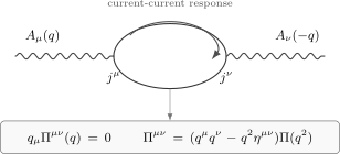
The vacuum current-current correlator generates the quadratic in-out functional of a background source. Gauge invariance requires the full polarization tensor, including contact terms, to be transverse; a causal response additionally requires the retarded prescription.
If is a background gauge field, vector gauge invariance means
Infinitesimally,
Since is arbitrary,
Differentiating once more with respect to and setting gives
In momentum space,
This is the transverse Ward identity.
Tensor structure and local counterterms
Section titled “Tensor structure and local counterterms”Lorentz invariance constrains the parity-even two-point tensor to be
Transversality gives
so . Hence
In Euclidean signature the same structure is
The local part must also be transverse if the vector current is gauged. For example,
shifts the polarization tensor by a local transverse polynomial,
where the sign follows from the displayed and the inherited inverse Fourier transform. By contrast,
would contribute and is not transverse. A local photon mass term is forbidden by exact gauge invariance.
A useful checklist is: nonlocal terms can carry physical long-distance information, while local transverse terms encode scheme choices and counterterms. Local non-transverse terms are allowed only when the source is not gauged or when the symmetry is explicitly broken.
This distinction matters later in two dimensions. A massless fermion loop can generate
This behaves like a mass term after gauge fixing, but it is nonlocal and transverse. It is therefore compatible with gauge invariance.
Ward contraction of the one-loop bubble
Section titled “Ward contraction of the one-loop bubble”For a Dirac fermion with vector current
write the raw quadratic Dirac kernel and its Feynman inverse as
Thus as a boundary-value identity, whereas . The raw kernel is not the literal inverse of the contraction . Expanding the fermion determinant, up to an -independent constant, gives the regulated loop
where the regulator and local completion are kept until the Ward identity is imposed. Contract with . Since
the contracted bubble becomes
Using inside the trace, together with cyclicity, gives a difference of two one-propagator integrals. In terms of it is
If these integrals were absolutely convergent, the second term could be shifted by , and the difference would vanish. But the individual integrals are ultraviolet divergent. Shifting a divergent integral is not a harmless algebraic step; it is a statement about the regulator.
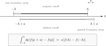
For a regulated divergent integral, shifting the integration variable removes one boundary strip and adds another. Their difference is the elementary origin of local surface terms in Ward-identity manipulations.
The one-dimensional analog is
For small ,
If vanishes at both ends, the boundary term disappears. If approaches different limits, the boundary term survives. A divergent loop integral can behave the same way.
The lesson is not that gauge Ward identities are unreliable. It is that Ward identities are statements about regulated composite operators. A gauge-invariant regulator and a gauge-invariant counterterm prescription define the local terms so that
If another classical symmetry is incompatible with this choice, that other symmetry becomes anomalous. This is why the anomaly is often visible as a finite “surface term” in a formally linearly divergent integral.
Vector and axial currents in two dimensions
Section titled “Vector and axial currents in two dimensions”In two dimensions the axial current is dual to the vector current. With the convention used on the previous page,
Suppose vector gauge invariance fixes the current-current correlator to be
For one massless Dirac fermion with the covariant unit-current normalization,
The vector Ward identity is automatic:
Now dualize one index to form the axial-vector correlator,
Its divergence is
because . Equivalently,
Thus a nonzero transverse vector kernel implies a nonzero axial divergence. With the source term , the in-out source expansion gives . In position space, for one positively charged unit Dirac fermion, this gives
The regulator has preserved vector gauge invariance. The axial current is anomalous.
Chiral bubbles in light-cone variables
Section titled “Chiral bubbles in light-cone variables”The same conclusion can be seen without gamma-matrix traces. A massless Dirac fermion in two dimensions splits into right- and left-moving components,
The chiral currents are
The propagator has the distributional form
and the propagator is
The sign of the infinitesimal imaginary part is crucial. It is the remnant of the relativistic Feynman prescription after the massless propagator has been factorized into chiral pieces.
The sign requires both the contour integral and the determinant prefactor. Let be the raw chiral kernel; its source is because and . Expanding its determinant gives
The Hessian therefore has an overall . The other prefactor is the positive Cartesian momentum Jacobian . The factor in cancels the in , leaving the raw inverse denominator . For a positive temporary , the separated loop is
Perform the integral first and then take the common boundary value. A finite sign- deformation is useful for checking residues; it is not itself a covariant regulator defining all local contact terms.
For fixed , the two poles in the complex plane lie on the same side unless and have opposite signs. For , this happens only in the strip
In this strip the upper pole is , while the other pole is . Closing above, with positive orientation, gives
The remaining strip has width , so the two factors of fix the sign:
For , the strip is and the upper pole comes from the second denominator. The contour integral is ; multiplication by the positive strip width gives the same boundary value. Exchanging the two chiralities then yields, away from the null cone,
Distributionally these are and with the common prescription specified above. Both chiralities have the same sign and magnitude. The full-sum source components and the Cartesian measure together fix this normalization; converting only one of them gives a wrong factor.
At separated points, the mixed right-left correlator vanishes,
The figure separates the support argument from the determinant phase. Follow the strip first, then the two factors of that determine the signed coefficient.
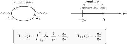
For and non-null external momentum, opposite-side poles restrict the loop to . The contour contributes in the boundary limit; the determinant contributes another and the Cartesian Jacobian is , giving . The strip is schematic, not to scale; finite checks the contour before its boundary limit.
The nonlocal ratios and are robust. A local counterterm cannot change them. What a local counterterm can change is the mixed component .
Gauge-invariant completion in two dimensions
Section titled “Gauge-invariant completion in two dimensions”For the unrescaled projectors and Cartesian measure used above, and . The global source convention therefore gives the exact coupling
The separated chiral bubbles give
Under the vector gauge transformation
the negative-momentum leg varies with the opposite phase. Varying both legs and then relabeling in one term gives the local variation
This can be canceled by the local contact term
Indeed, its two-leg variation is . Thus the gauge-invariant quadratic effective action is
Equivalently,
where the full-sum gauge-invariant momentum combination is
The negative argument also reverses the momenta:
This minus sign produces the negative same-chirality terms when the bilinear is expanded. The two mixed terms become equal after integration and relabeling, not at an arbitrary individual momentum. Exercise 4 checks the expansion and a sign-sensitive timelike example.
With the inherited inverse Fourier transform and the coordinate components of lesson 23, . This gives an explicit round trip from the full-sum notation to the curvature two-form.
The same round trip fixes the normalization without a convention-dependent remainder:
so reproduces the covariant kernel .
In the next figure, denotes the sum of the two unsigned diagonal bilinears and the sum of both mixed bilinears:
Inspect the signs in : the positive contact completes the negative chiral pieces into the curvature bilinear.
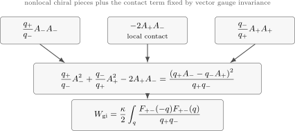
For the page’s full-sum sources and common boundary prescription, and . Their variations cancel and . The negative-momentum argument is essential. This schematic sequence uses and the bilinears defined in the text; it does not represent an ordinary square at one momentum.
This is the cleanest way to see why the mixed polarization component is subtle. The separated diagram gives . The full gauge-invariant distribution contains a local contact term. Without it, the vector Ward identity fails. This is the concrete two-dimensional example of the general warning at the start of the page: separated-point correlators and full response kernels are not the same object.
The expression should be read as a nonlocal quadratic functional. After the explicit factor-four translation above, it is the two-dimensional version of . It is gauge invariant because it is written in terms of the curvature combination, but it is not the same as a local Proca mass .
If is made dynamical, the induced action contains the transverse projector
The sign matters as well as transversality. With the rescaled Maxwell term , the transverse inverse coefficient is
For a timelike mode with , : the same quadratic kernel is . Reversing the induced coefficient would instead give a negative mass squared even though the tensor remains transverse. This is the massless Schwinger-model mechanism. The physical massive mode and the zero-flux, infinite-line assumptions are developed in the bosonization calculation.
Regulator choice and the anomaly
Section titled “Regulator choice and the anomaly”A gauge-invariant Pauli–Villars definition makes the symmetry choice explicit and checks the normalization without relying on the chiral split. Start with a small positive physical mass and a large regulator mass , using the same vector coupling in both determinants:
Normalize by the corresponding zero-source ratio. Combine the two loop integrands before removing the regulator or shifting the loop momentum. Their leading ultraviolet terms cancel. The massless physical limit is taken after the regulated calculation.
For a nonzero Euclidean momentum , the Dirac trace, a Feynman parameter , and the convergent momentum integral give
This regulated, integrated tensor is already transverse. As , the first integral tends to ; the second is bounded above by and vanishes as . Thus
The Wick rotation carries the source one-form with it: gives and . Together with on the rotated contour, this maps the positive Euclidean coefficient to the positive Lorentzian coefficient used above. This is the vector-gauge-preserving mass limit evaluated in Morais and Mota 2009, § V, p. 8, Eqs. (42)–(48), PDF. It also shows why a local contact cannot repair the wrong sign of the nonlocal term.
The heavy regulator preserves vector gauge invariance, but its mass couples left and right movers. It therefore breaks the axial rotation that assigns opposite phases to and . When the physical mass has gone to zero, the surviving regulator contribution leaves the exact vector Ward identity
and the anomalous axial Ward identity
The anomaly is the finite trace left by the ultraviolet regulator in the contact term of a current-current correlator.
This viewpoint is deliberately operational. To compute a current correlator, first regulate it; then add the local counterterms required by the symmetry you insist on preserving; only then ask whether another classical Ward identity still holds.
Bridge to many-body response
Section titled “Bridge to many-body response”The contour argument in the chiral bubble will reappear in the next page. A nonrelativistic Fermi gas has particle and hole propagators whose poles can lie on opposite sides of the energy contour. The corresponding loop is nonzero only in restricted kinematic regions near the Fermi surface. The same analytic idea underlies density response, current response, and Fermi-surface instabilities.
In relativistic field theory, current correlators organize Ward identities and anomalies. In many-body theory, related kernels describe the response of a filled sea. The state and causal prescription must be chosen for that problem: a vacuum time-ordered loop cannot simply be relabeled as a retarded density response. In both settings, poles, contact terms and symmetry constrain the calculation.
Summary
Section titled “Summary”The time-ordered current kernel is the quadratic Hessian of the connected in-out functional with respect to a background source. For a non-anomalous vector current,
Lorentz invariance then gives the transverse structure
At one loop, the Ward contraction reduces to a difference of shifted integrals. If the integrals are divergent, the shift can leave a finite boundary term. A regulator and local counterterms are therefore part of the definition of the Ward identity.
In two dimensions, chiral current bubbles give
The full-sum convention gives and the positive covariant unit-current coefficient . The separated mixed correlator vanishes, but vector gauge invariance requires the positive mixed contact term in this normalization. The completed answer is
Preserving vector gauge invariance forces the axial Ward identity to contain the anomaly.
Common pitfalls
Section titled “Common pitfalls”Ignoring contact terms. The separated-point diagram is not the full polarization tensor. The missing term can be local and still required by a Ward identity.
Shifting divergent integrals without saying how they are regulated. A formal loop-momentum shift is safe only for convergent integrals or for regulators that make the shift legitimate.
Mistaking a transverse nonlocal term for a forbidden local mass. The two-dimensional induced action behaves like a mass after gauge fixing, but it is written with a transverse projector and is gauge invariant.
Losing a Fourier or loop phase. The argument reverses the momentum in . The residue supplies one and the fermion determinant supplies another. Transversality alone will not detect reversing the entire induced action; the covariant normalization and positive mass pole do.
Trying to conserve vector and axial currents simultaneously in the regulated theory. For the massless two-dimensional Dirac fermion, preserving vector gauge invariance forces the axial current to be anomalous.
Comparing absolute light-cone coefficients before translating conventions. The ratios and are invariant under harmless rescalings, but their prefactor is not. Compare the covariant tensor or explicitly translate coordinates, currents, sources, and the measure.
Exercises
Section titled “Exercises”Exercise 1: Derive transversality from source gauge invariance
Section titled “Exercise 1: Derive transversality from source gauge invariance”Starting from
show that invariance under implies . Keep the transformation of the negative-momentum leg and use .
Solution
The variation of the quadratic term is
In the second term, relabel , exchange and , and use the stated symmetry. The reversed momentum supplies the extra minus sign, so the two contributions add:
Since and are arbitrary,
Exercise 2: Construct the transverse tensor structure
Section titled “Exercise 2: Construct the transverse tensor structure”Assume Lorentz invariance and write
Use to determine the transverse form.
Solution
Contracting with gives
For arbitrary , transversality requires
Therefore
Renaming gives the standard tensor structure.
Exercise 3: Locate the chiral bubble support strip
Section titled “Exercise 3: Locate the chiral bubble support strip”For , consider the chiral bubble integral
Explain why only the strip contributes. Replace temporarily by and evaluate the phase and coefficient of , integrating over first. Which additional factors convert it into ?
Solution
For fixed , the poles in the plane are
If and have the same sign, the poles lie on the same side of the real axis, so the contour can be closed in the empty half-plane and gives zero.
For , the signs are opposite only when
In that strip the upper pole is . Its residue is ; closing above gives after the integration factor. The remaining integral gives
Hence
The extra is from the determinant Hessian and the extra is the Cartesian momentum Jacobian. The last ratio has the common boundary prescription; finite only defines this intermediate contour test.
Exercise 4: Complete the chiral bubbles gauge-invariantly
Section titled “Exercise 4: Complete the chiral bubbles gauge-invariantly”Starting from , derive its expression at and show that
Check the sign for with and , and compare with .
Solution
Reversing the argument reverses the full-sum momenta:
Multiplying by gives negative diagonal terms and , and positive mixed terms. Dividing by yields the stated expression. The mixed terms combine into twice either one only after integration and relabeling.
For the timelike example, , and . Therefore
The covariant expression agrees because . Replacing the opposite-momentum bilinear by an ordinary square would instead give . With the Maxwell term, the correct sign yields and the positive pole .
Exercise 5: Recover the axial divergence from vector response
Section titled “Exercise 5: Recover the axial divergence from vector response”Let
Show that
Solution
Compute
The second term vanishes because
Thus
Using , we obtain
References
Section titled “References”- C. W. Morais and A. L. Mota, “Momentum Space Regularizations and the Indeterminacy in the Schwinger Model,” International Journal of Modern Physics A 26 (2011) 1991–2006, DOI: 10.1142/S0217751X11053067. Preprint: arXiv:0910.4322v1 (2009), Open PDF; page and equation locators above refer to this version.
- W. Pauli and F. Villars, “On the Invariant Regularization in Relativistic Quantum Theory”, Reviews of Modern Physics 21 (1949) 434–444.
- J. Schwinger, “Gauge Invariance and Mass. II”, Physical Review 128 (1962) 2425–2429.
- Y. Takahashi, “On the Generalized Ward Identity”, Il Nuovo Cimento 6 (1957) 371–375.
- J. C. Ward, “An Identity in Quantum Electrodynamics”, Physical Review 78 (1950) 182.
Further reading
Section titled “Further reading”- S. Coleman, Lectures of Sidney Coleman on Quantum Field Theory, B. Gin-ge Chen, D. Derbes, D. Griffiths, B. Hill, R. Sohn, and Y.-S. Ting (eds.), World Scientific (2019), lectures on Ward identities, regularization, and two-dimensional fermions.
- A. M. Polyakov, Gauge Fields and Strings, Harwood Academic Publishers (1987), discussions of two-dimensional field theory, gauge invariance, and anomalies.
- M. D. Schwartz, Quantum Field Theory and the Standard Model, Cambridge University Press (2014), chapters on vacuum polarization, Ward–Takahashi identities, and anomalies.
- M. Srednicki, Quantum Field Theory, Cambridge University Press (2007), sections on vacuum polarization, QED Ward identities, and anomalies.
- S. Weinberg, The Quantum Theory of Fields, Vols. I–II, Cambridge University Press (1995–1996), chapters on current correlators, gauge-theory renormalization, and anomalies.
- A. Zee, Quantum Field Theory in a Nutshell, 2nd ed., Princeton University Press (2010), discussions of vacuum polarization, two-dimensional fermions, and anomalies.