

Critical Propagators and the Upper Critical Dimension
The previous page derived the continuum scalar field from the Ising model by an exact Hubbard–Stratonovich transformation. The Gaussian part of that field theory already knows a lot: it knows which momentum mode becomes soft, how the correlation length diverges, and why the two-point function near criticality has the universal form of a massive free scalar propagator.
This page asks the next question. Once the continuum action contains an interaction such as , when is the Gaussian propagator trustworthy? The answer is not simply “when is small.” Near a critical point the correlation length becomes large, so fluctuations are sampled over larger and larger regions. The true expansion parameter is a scale-dependent one,
Thus the Ising interaction becomes less important at long distances for , marginal for , and more important for . The number
is the upper critical dimension. For the ordinary short-range scalar transition, bulk mean-field exponents hold above it. Below it, the quartic interaction destabilizes the Gaussian fixed point. Near four dimensions the Wilson–Fisher fixed point provides a controlled replacement. Power counting by itself does not establish that a finite-temperature transition exists in every dimension.
Required background. Hubbard–Stratonovich transformation and the continuum field supplies the lattice quadratic kernel, the auxiliary-field propagator, and the continuum action used below.
Critical modes of a lattice kernel
Section titled “Critical modes of a lattice kernel”Start with a translation-invariant ferromagnetic interaction. In the spin language one may write schematically
with real even couplings , nonnegative off-site couplings, and finite range or exponential decay. These hypotheses make analytic and ensure . Assume also a nondegenerate isotropic quadratic maximum; an anisotropic positive stiffness would give a tensor of correlation lengths. Its Fourier transform is
The Hubbard–Stratonovich Gaussian propagator from the previous page has the form
up to a smooth nonzero normalization factor. The important information is the zero of the inverse propagator. In the Gaussian or random-phase approximation, an instability occurs when some eigenvalue of the interaction kernel reaches
For a ferromagnet, the largest value of is at , so
If the maximum is instead at a nonzero wavevector , the soft field is not the uniform magnetization. The continuum expansion must be made around , which describes antiferromagnetic or modulated order. This is the same mathematical mechanism with a different ordering wavevector.
Under the stated analyticity and isotropy assumptions,
Define the reduced distance from the Gaussian critical point by
On the disordered side, . Then
Write the smooth numerator to leading order as and set . Dividing the whole denominator by gives the Ornstein–Zernike form
Thus on the disordered side. For this quadratic propagator, is the inverse second-moment length and also the continuum pole mass:
Therefore the Gaussian theory predicts
This is the mean-field value .
The figure separates the stiffness , which sets the length, from the field amplitude .
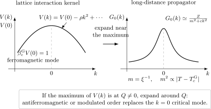
The soft mode lies at the maximum of the lattice kernel. On the disordered side of an isotropic ferromagnetic Gaussian instability, , , and . The quadratic propagator has ; a different ordering wavevector requires expansion around that wavevector. The kernel curve is schematic, not a quantitative lattice spectrum.
For the nearest-neighbor hypercubic Ising model,
At small ,
Thus
The Gaussian critical value is
and
This last expression is the dimensionless spin susceptibility of the Gaussian approximation, before canonical field normalization. The exact critical point is shifted by fluctuations in dimensions where the interaction is important. The Gaussian calculation nevertheless identifies the soft mode and the analytic structure around it. The superscript on is essential; is not the exact nearest-neighbor Ising critical coupling.
Position-space propagator and the correlation length
Section titled “Position-space propagator and the correlation length”For the canonically normalized field (), the continuum Gaussian propagator at a noncoincident point is
The formulas in this section use the continuum Green distribution, with the ultraviolet regulator removed at . An abrupt finite momentum cutoff adds oscillatory long-distance tails, so one must not extract an exponential length from that cutoff artifact. Loop integrals later retain their stated cutoff. The distinction between the pole length, the second-moment length and sharp-cutoff ringing is explicit in Wilson and Kogut 1974, § 3, pp. 98–99.
At criticality, , dimensional analysis alone gives
for . With the normalization above, the exact coefficient is
Away from criticality,
where is a modified Bessel function and . This formula has two important limits. For and distances much shorter than ,
so the system looks critical. In the corresponding behavior is logarithmic:
The massless field has no finite translation-invariant covariance of this form in two dimensions, but the difference tends to as . For distances much longer than ,
so correlations are exponentially suppressed.
The susceptibility is the zero-momentum two-point function,
Since , Gaussian theory gives
Thus . At this level the anomalous dimension is also zero, because at criticality
The central issue is whether interactions preserve these exponents.
Dyson equation and critical mass tuning
Section titled “Dyson equation and critical mass tuning”The continuum action near the Ising critical point is
The dots include higher even powers and higher derivatives. For the present page the leading interaction is the quartic term. Perturbatively, the exact two-point function is organized by one-particle-irreducible self-energy insertions:
The physical susceptibility is not fixed by the bare parameter . At zero momentum the exact inverse propagator gives
The critical point is the value of the microscopic parameters for which diverges,
Thus criticality is a tuning condition. The bare mass must cancel the fluctuation correction:
Near the critical point it is often cleaner to subtract the critical value:
This formula is the statistical-mechanics version of mass renormalization. The lattice cutoff regulates ultraviolet divergences; it does not remove critical infrared singularities. The separation between the physical susceptibility scale and the microscopic bare mass is still essential. When the coefficient of has been normalized to one, we may abbreviate as and identify it with , as in the convention note.
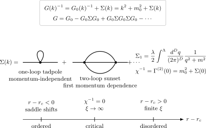
Self-energy insertions shift the inverse propagator. The critical point is defined by , not by the naive vanishing of the bare mass. With , expanding produces alternating signs. In theory the one-loop tadpole shifts ; momentum-dependent corrections begin at two loops.
Using a propagator with the renormalized scaling mass —equivalently, reorganizing perturbation theory around the physical quadratic term—the one-loop tadpole gives
The factor follows from the conventional normalization. Other normalizations of the quartic term move this numerical factor but not the scaling.
Write
where
is the area of the unit -sphere. The ultraviolet behavior is
This cutoff-dependent constant shifts the critical temperature. It is not universal. The universal question is how the remaining long-distance part behaves as .
For ,
For ,
For , the leading small- correction is analytic in once the cutoff is kept fixed:
For noninteger , a subleading nonanalytic term proportional to can also occur; it does not overturn the leading comparison with . At even dimensions further logarithms appear in subleading orders.
The borderline behavior at is the first warning that four dimensions are special. The next section gives a cleaner and more general explanation.
Power counting at the Gaussian fixed point
Section titled “Power counting at the Gaussian fixed point”At criticality the Gaussian action is
Under the coordinate dilation
the derivative scales as
and the measure scales as
The transformed field that leaves invariant is
Equivalently, the engineering dimension of the scalar field is
Now consider the quartic interaction
The operator has dimension
Since the action is dimensionless,
Therefore
This single equation encodes the upper critical dimension:
At a length scale , the associated dimensionless coupling is
Thus as for . This is the precise sense in which mean-field theory becomes exact at the longest distances above four dimensions. For , grows with , so the Gaussian approximation eventually breaks down no matter how small the microscopic coupling was.
At , power counting alone cannot decide the fate of . Quantum or statistical fluctuations generate logarithms, and the next page will turn those logarithms into a renormalization-group flow.
Position-space Ginzburg test
Section titled “Position-space Ginzburg test”There is a useful way to see the same result in a correlation function. Initially keep a UV regulator of length , a positive mass as an IR regulator, and, if a finite box is used, its length . Work at separations . A finite periodic box alone would leave the massless zero mode unregulated. For , the critical Gaussian power law in that range is
The composite operator is the continuum representative of the local energy-density perturbation. After subtracting its expectation value, its Gaussian connected two-point function behaves as
The subscript is essential: the raw expectation also contains . At a regulator where coincident fields exist, Wick’s theorem gives that disconnected term plus the two cross contractions displayed above.
Consider the first-order graph in which all four fields at one interaction vertex contract with the two composite insertions. Expanding gives a minus sign. There are contractions, cancelling , so this particular graph is
The propagators and integral here first retain the regulators. Tadpole graphs, the adjustment of the mass and renormalization of the composite operator are separate terms in the full connected correlator.
To isolate a contribution at the observation scale, restrict the vertex to
This region stays away from both endpoints and from infinity; its shape is fixed under . Its volume scales as
and each of the four propagators is of order . The magnitude of the restricted graph therefore scales as
Here , as appropriate to the stable quartic potential. Its relative magnitude is
This is the same dimensionless coupling found by power counting. It is a scale-local estimate, not a claim that the full massless insertion is finite in every dimension.
Indeed, removing both regulators in that full graph imposes two different tests. Near either endpoint, a radial distance gives an integral , finite only for . Far from both endpoints, the radial integral is , finite only for . Thus the unregulated graph converges precisely in
At the endpoints the corresponding divergence is logarithmic. UV counterterms do not remove the far-distance divergence at ; keep the mass or volume regulator there. The engineering argument for remains valid outside this convergence window, whereas this unregulated massless graph does not.
A finite three-dimensional check
Section titled “A finite three-dimensional check”For and , and the full insertion is convergent. A Feynman parameter evaluates the required convolution:
The shift is . Hence this graph, with the stated normalization, gives
This checks the sign, numerical combinatorics and the power for this graph. It does not replace the other first-order contributions to the full renormalized composite correlator. The figure summarizes the regional estimate and its separate convergence qualification.
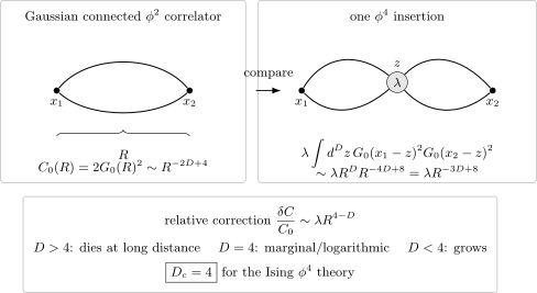
For in the Gaussian scaling range, the connected free composite correlator is . Restricting the quartic vertex to gives . The full massless graph instead requires ; outside that window retain the appropriate regulators and renormalization terms. Lines and vertex positions are schematic.
The same estimate is often called the Ginzburg criterion. Evaluate the dimensionless coupling at the correlation length:
As , . Therefore:
- for , , so the Gaussian or mean-field approximation becomes asymptotically reliable;
- for , is marginal and receives logarithmic corrections;
- for , , so critical fluctuations invalidate mean-field exponents.
These statements concern the growth of the Gaussian expansion parameter where a continuous transition exists. They do not derive the interacting exponents or establish a transition in every dimension. For small positive in , the Wilson–Fisher fixed point is a controlled replacement; see Wilson and Fisher 1972, pp. 241–243.
The random-walk meaning of 4 equals 2 plus 2
Section titled “The random-walk meaning of 4 equals 2 plus 2”There is a beautiful interpretation of the number four. The Gaussian propagator has the Schwinger representation
Fourier transforming gives
The parameter behaves like the length, or proper time, of a Brownian path. At criticality , the exponential factor
says that paths contributing to a displacement typically have
Thus a free critical propagator is geometrically like a random walk of fractal dimension .
The quartic interaction couples two such walks when they meet. The elementary intersection-dimension estimate says that two sets of fractal dimension have a positive-dimensional intersection when
The borderline is
This is the geometric version of the upper critical dimension. Above four dimensions, intersections of two long independent walks are sufficiently sparse that the local interaction becomes irrelevant; below four dimensions they proliferate and reshape the long-distance theory. At the borderline, the estimate is marginal and logarithms decide the result. This is an interpretation of the power counting, not a substitute for the renormalization-group argument.
This random-walk viewpoint will reappear later in the course when field-theoretic propagators are related to sums over paths, and eventually when random surfaces enter the discussion.
Mean field above four dimensions and its caveat
Section titled “Mean field above four dimensions and its caveat”For , the long-distance critical two-point function is Gaussian:
The critical exponents take their mean-field values:
However, one should be careful with the phrase “the interaction is irrelevant.” The quartic coupling is irrelevant at the Gaussian fixed point in the renormalization-group sense, but it is still needed to stabilize the ordered phase. If , the potential
is unbounded unless the quartic term is kept. Thus is dangerously irrelevant above four dimensions: it does not change the leading long-distance two-point critical behavior, but it enters thermodynamic quantities such as the magnetization amplitude in the ordered phase.
This subtlety is one reason critical phenomena are more delicate than a first reading of power counting suggests. Power counting identifies which fixed point is stable; it does not automatically tell us which amplitudes and scaling relations remain ordinary. In particular, bulk mean-field exponents hold for , but hyperscaling and naive finite-size scaling fail because they are sensitive to the dangerously irrelevant coupling.
Example: the one-loop mass shift
Section titled “Example: the one-loop mass shift”Let us make the mass-renormalization statement concrete. In the symmetric phase, use
At one loop,
Using rather than in the internal line is a convenient self-consistent notation; replacing it by the zeroth-order mass changes the result only beyond the displayed order away from the critical infrared singularity.
The critical bare mass is obtained by setting :
Therefore
The first term is the experimentally or microscopically tunable distance from the critical point. In a thermal system it is proportional to after nonuniversal normalization. The second term is the fluctuation correction.
For , the bracket is proportional to times a cutoff-dependent coefficient, so it can be absorbed into a finite renormalization of the slope relating to . Mean-field scaling survives.
For , the bracket contains
so logarithmic corrections appear.
For , the bracket contains a nonanalytic contribution
This term becomes more singular than as . At and below , even has an infrared divergence, so the subtraction must be reformulated. In either case ordinary perturbation theory around the Gaussian point has lost control in the infrared. Near four dimensions, the expansion repairs this by moving the expansion point from the Gaussian fixed point to a nearby interacting fixed point.
Summary
Section titled “Summary”The lattice interaction kernel determines which mode becomes critical. For a ferromagnet,
and the Gaussian propagator near the critical point takes the universal form
At criticality for ,
so Gaussian theory predicts , , and .
Interactions shift the critical point through the self-energy:
After normalizing the coefficient, .
The one-loop tadpole gives
so the bare mass must be tuned against fluctuation corrections to reach .
The quartic coupling has engineering dimension
Equivalently, its dimensionless strength at length scale is
Thus
is the upper critical dimension of the Ising theory. Above four dimensions the Gaussian fixed point controls the critical exponents. Below four dimensions the quartic interaction grows at long distances, and the correct critical theory is interacting.
Common pitfalls
Section titled “Common pitfalls”Calling the Gaussian instability exact. The condition is not generally the exact critical temperature. It is the point at which the quadratic approximation becomes unstable; fluctuations shift it.
Equating every definition of mass. Exactly, . It equals only after normalizing the coefficient, while the exponential correlation length comes from the nearest complex-momentum singularity. These definitions share a critical exponent but can differ by finite factors.
Discarding the tadpole as a divergent nuisance. In a lattice statistical model it is finite, but it still changes the relation between microscopic temperature and physical correlation length. Renormalization is already present conceptually before taking a continuum cutoff to infinity.
Mistaking power counting for the full RG. Power counting identifies as the marginal dimension. At exactly four dimensions logarithms decide the flow; below four dimensions the Wilson–Fisher fixed point replaces the Gaussian fixed point.
Dropping the quartic term above four dimensions. It is irrelevant for leading bulk critical exponents but still stabilizes the ordered phase and affects amplitudes, hyperscaling, and finite-size scaling. This is the standard dangerously irrelevant caveat.
For the renormalization-group organization of the upper-critical-dimension argument, continue to Gaussian and Wilson–Fisher Fixed Points in the Library. It distinguishes the Gaussian power counting used here from the interacting fixed point reached below four dimensions.
Exercises
Section titled “Exercises”Exercise 1
Section titled “Exercise 1”Let
and suppose
Assuming , show that near the propagator can be written in the form
Find in terms of , , and up to an overall normalization convention.
Solution
Using the small- expansion,
Define
Then
Factor out from the denominator:
Thus
Since , near the Gaussian transition
on the disordered side. In terms of temperature this is proportional to , up to a positive nonuniversal constant.
Exercise 2
Section titled “Exercise 2”Use dimensional analysis to show that
scales as for and , with the Fourier integral understood as the continuum Green distribution. Explain why one cannot set in the resulting coefficient to obtain a finite constant covariance.
Solution
Let and rescale the integration variable by
Then
Therefore
For the infrared integral is locally integrable. At , removing the UV regulator in the distributional sense leaves a dimensionless coefficient independent of . Thus
For the standard normalization gives
At the coefficient has a pole and the massless infrared integral diverges. With , the small- result is logarithmic; the difference between two nonzero separations tends to . A scale-independent finite constant would miss that dependence.
Exercise 3
Section titled “Exercise 3”For
show by power counting that has a UV divergence proportional to for . What happens at ?
Solution
Using spherical coordinates,
For ,
up to the infrared lower limit. Therefore
At , the integral becomes
which is logarithmic. In the massless theory this logarithm is also infrared divergent. With nonzero , the denominator cuts off the infrared region and produces a logarithm of .
Exercise 4
Section titled “Exercise 4”Find the engineering dimensions of and in
Use them to identify the upper critical dimension.
Solution
The action is dimensionless. Since and , the kinetic term gives
Hence
The quartic interaction gives
Substituting the field dimension,
The coupling is dimensionless when
Therefore the upper critical dimension of the interaction is
For , and the interaction is irrelevant at the Gaussian fixed point. For , and it is relevant.
Exercise 5
Section titled “Exercise 5”In the Gaussian scaling range for , let
Define the connected composite correlator
For , estimate the graph in which all four vertex fields contract with the endpoints, restricting the vertex to defined above. Show that its relative magnitude scales as . Give the convergence window if one instead integrates this graph over all space with the massless continuum propagator.
Solution
The Gaussian correlator is
The specified restricted graph is
For a scaling estimate at separation , the integration region has volume , and each propagator contributes a factor . Since there are four propagators,
Therefore
This relative magnitude decreases with for , grows for , and is marginal by power counting for . Without the restriction, endpoint convergence requires to converge, while convergence at infinity requires . Thus the full massless graph is finite only for . Subtracting the disconnected expectation does not cure these separate UV or IR singularities.
Exercise 6
Section titled “Exercise 6”Use the Schwinger representation
to show that a critical Gaussian propagator describes paths with typical length for endpoint separation .
Solution
Fourier transforming the Schwinger representation gives
The Gaussian momentum integral is
Thus
At criticality . The exponential factor suppresses , because then is large. The power suppresses very large in dimensions where the integral is convergent. The natural scaling variable is
Therefore the dominant path length scales as
This is the Brownian scaling relation: the path has fractal dimension .
References
Section titled “References”- Wilson, Kenneth G., and Michael E. Fisher. “Critical Exponents in 3.99 Dimensions.” Physical Review Letters 28, no. 4 (1972): 240–243. DOI.
- Wilson, Kenneth G., and John Kogut. “The Renormalization Group and the Expansion.” Physics Reports 12, no. 2 (1974): 75–199. DOI.
Further reading
Section titled “Further reading”- Cardy, John. Scaling and Renormalization in Statistical Physics. Cambridge Lecture Notes in Physics 5. Cambridge: Cambridge University Press, 1996. Chapters 2–4.
- Ginzburg, Vitaly L. “Some Remarks on Phase Transitions of the Second Kind and the Microscopic Theory of Ferroelectric Materials.” Russian original, Fizika Tverdogo Tela 2, no. 9 (1960): 2031–2043. Author’s institutional bibliography, item 374.
- Goldenfeld, Nigel. Lectures on Phase Transitions and the Renormalization Group. Frontiers in Physics 85. Reading, MA: Addison-Wesley, 1992. Chapters 4–6.
- Polyakov, Alexander M. Gauge Fields and Strings. Contemporary Concepts in Physics 3. Chur: Harwood Academic Publishers, 1987. Chapters 1–3 and 9.
- Zinn-Justin, Jean. Quantum Field Theory and Critical Phenomena. 5th ed. Oxford: Oxford University Press, 2021. Chapters 14–17.