

In–Out, In–In, and Schwinger–Keldysh Functionals
The previous page described vacuum decay through the vacuum persistence amplitude. That already forced a distinction that is easy to miss in ordinary perturbation theory. A quantity such as
is a transition matrix element. It is the right object for scattering amplitudes, the ordinary Feynman effective action, and vacuum-to-vacuum transitions. It is not, by itself, the expectation value measured by an observer who prepares a state in the past and asks what an operator is at time .
This page develops the real-time formalism that keeps that distinction honest. The ordinary Feynman, or in–out, formalism fixes both an initial and a final vacuum. The in–in, or Schwinger–Keldysh, formalism fixes only the initial state and evolves both the ket and the bra. The reward is causality: the response of an operator at time depends only on the past of , even though Feynman propagators themselves are not retarded functions.
The conceptual slogan is short:
Required background. Vacuum persistence and its imaginary part explains why a vacuum-to-vacuum amplitude need not have unit modulus, while the Feynman propagator and its prescription supplies the in–out boundary condition used below.
Helpful background. Hyperbolic equations and causal propagators reviews causal support and retarded or advanced Green operators.
| Formalism | Boundary data | What it naturally computes | Typical Green function |
|---|---|---|---|
| in–out | initial vacuum and final vacuum | scattering amplitudes, vacuum persistence, ordinary effective action | Feynman propagator |
| in–in / Schwinger–Keldysh | initial density matrix only | expectation values, currents, particle number, backreaction | retarded and Wightman functions |
The table is a good diagnostic while reading the rest of this page: whenever the desired answer is a number measured at time in a prepared state, the in–in column is the safer starting point.
Time evolution and vacuum persistence
Section titled “Time evolution and vacuum persistence”Work first at finite preparation and observation times, with well-defined unitary evolution, a Hermitian interaction and real probes. In the interaction picture, let
for . Infinite time bounds below denote an asymptotic limit only when it exists; they do not prepare a state by themselves. For local perturbation theory one can instead keep smooth switching of compact spacetime support, suppressed in the displayed interaction integrals. Removing that switching is a separate infrared limit. When asymptotic vacua exist, denote the prepared initial vacuum by . Its future evolution is
Its overlap with the future vacuum is the vacuum persistence amplitude,
A convenient notation is
The functional is the sum of connected vacuum bubbles. For a nonzero vacuum overlap and a common prescription in numerator and denominator, normalized Feynman correlators cancel disconnected vacuum bubbles order by order:
When the vacuum is stable, is a phase. When the vacuum can decay, or when an external field can create particles, . Writing
one finds
Thus an imaginary part of the in–out effective action is not an inconsistency. It says that the vacuum-to-vacuum channel is not closed. Probability has gone into other final states.
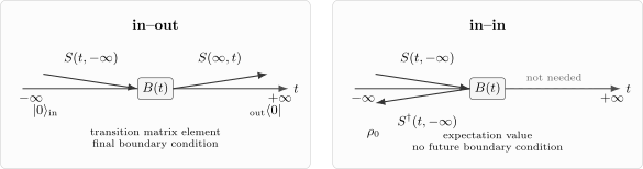
The in–out object evolves from the past to the future and projects onto a final vacuum. The in–in object evolves a ket forward to the operator and evolves the bra back along the conjugate path, so it is an expectation value in the state prepared in the past.
In–out matrix elements are not expectation values
Section titled “In–out matrix elements are not expectation values”Let be a Heisenberg operator, represented in the interaction picture by inserting the appropriate evolution operators. The in–out quantity associated with the ordinary Feynman functional is
The factor is the giveaway. This expression knows about the future boundary condition. It is a transition matrix element between an initial vacuum and a final vacuum, divided by their overlap.
The actual expectation value in the state prepared at is instead
No evolution beyond is needed. The ket evolves forward to ; the bra evolves backward from to the same initial density matrix. In a pure state this is simply the ordinary expectation value
The distinction is invisible in some equilibrium calculations because the same Feynman diagrams are often repurposed after analytic continuation or after extracting on-shell amplitudes. It becomes essential for time-dependent backgrounds, vacuum decay, cosmology, transport, particle production, and any problem where the question is “what does the system do?” rather than “what is the transition amplitude between two vacua?”
The closed time path
Section titled “The closed time path”The Schwinger–Keldysh construction encodes the in–in expression as a path integral on a doubled time contour. Prepare a positive density operator with at finite time , choose a return time later than every operator insertion, evolve forward on a branch, and evolve backward on a branch. Assume the stated expectations exist in this state. The return time is bookkeeping, not a future boundary condition; it may be moved without changing observables as long as it remains later than all insertions. The finite initial-density construction is given in Berges 2004, arXiv v1, § 3.1, pp. 29–30, PDF; closed-time-path grammar develops the initial-kernel representation. Fields on the two branches are denoted
Sources are also doubled. The closed-time-path generating functional is
For a pure initial state , cyclicity of the trace gives
In path-integral form,
The two fields are sewn together and integrated over at . The minus sign in front of is not optional: it is the complex-conjugate time evolution of the bra. A non-Gaussian also produces interaction vertices localized at the initial surface.
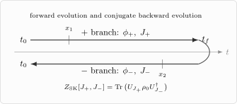
The Schwinger–Keldysh contour doubles the fields. The branch evolves forward with , while the branch evolves backward with . The two histories are sewn at any later than the latest insertion; equal sources then give .
The normalization property is crucial:
This identity assumes a normalized density matrix and a Hermitian source coupling, so that evolution with the common source is unitary. Closed-time-path vacuum bubbles then cancel against their conjugates. In the in–out formalism, vacuum bubbles exponentiate into . In the in–in formalism with equal sources, the corresponding closed contour gives unity. That is the diagrammatic reason the Schwinger–Keldysh formalism is naturally normalized for expectation values.
Four real-time propagators
Section titled “Four real-time propagators”Contour ordering produces four two-point functions. Define
For a translation-invariant vacuum initial state in a free scalar theory,
Here is time ordering and is anti-time ordering. With the Fourier convention of the course,
The mixed propagators are on shell. They are the real-time Wightman functions, and in cut diagrams they are the lines that cross from an amplitude to its complex conjugate. For a thermal or populated Gaussian state the same free spectral support remains, but the positive- and negative-frequency terms acquire occupation factors. For an interacting or nonstationary state, the compact vacuum momentum-space formulas above no longer apply even though the contour definitions do.
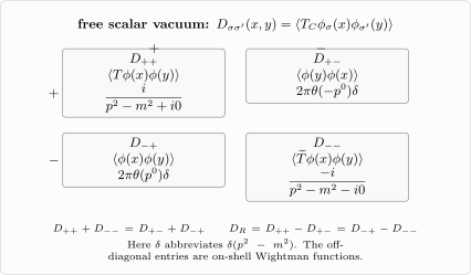
For the free scalar vacuum shown here, the doubled contour gives a matrix of real-time propagators. The diagonal entries are Feynman and anti-Feynman propagators; the off-diagonal entries are Wightman functions supported on the mass shell in momentum space.
These four functions are not independent. Since
and
one has, with a common prescription at coincident times,
The retarded function is the difference
The advanced partner is
At equal times, contact terms and the convention for must be treated consistently. Away from coincident points, these identities are purely algebraic. They show how causal response is built from Feynman and Wightman pieces so that the nonretarded parts cancel.
Branch signs and cut diagrams
Section titled “Branch signs and cut diagrams”Perturbation theory on the closed contour has a simple rule. A vertex on the branch carries the ordinary factor from . A vertex on the branch carries the complex-conjugate factor from . For example, if
then a vertex contributes
whereas a vertex contributes
Internal lines know which branches their endpoints live on:
The diagrammatic structure resembles the decomposition of a probability into an amplitude and a conjugate amplitude. The left side of a cut contains ordinary Feynman propagators, the right side contains complex-conjugate propagators, and the cut lines are on shell. Schematically,
and
Up to conventional factors of and , these are exactly the ingredients displayed by the Schwinger–Keldysh matrix. This is why closed-time-path perturbation theory is the natural language for inclusive probabilities, particle production, transport, and nonequilibrium evolution.
The Keldysh rotation
Section titled “The Keldysh rotation”The doubled fields are often reorganized into “classical” and “quantum” combinations,
Similarly define
The source term becomes
The physical limit of equal sources is
Define the connected functional by
This notation makes unitarity visible. The action difference
vanishes when , and the generating functional satisfies . An ordinary expectation value is obtained from the auxiliary difference source:
The response to the physical common source is
for the source and correlator conventions of this page. This makes the index logic precise: the observable comes from a derivative, while varying the physical source adds a derivative.
The same rotation organizes the two-point functions into
where
is the statistical correlator. It includes the mean product when ; subtract that product to obtain the centered covariance. The zero in the entry expresses closed-contour normalization. The rotation separates causal and statistical roles, not dynamics from state dependence: in an interacting theory and can also depend on the prepared state. The state-independent commutator of the free oscillator below is a special case. See Berges 2004, arXiv v1, § 3.4.1, pp. 35–36, and § 3.4.3, p. 40, Eq. (138), PDF.
Causal response from the closed contour
Section titled “Causal response from the closed contour”The simplest test is first-order perturbation theory. Let be a local observable with no explicit dependence on the perturbation, and let
The in–in expectation value is
Expanding to first order gives
Therefore
This is a retarded formula: the upper limit is . In a local relativistic continuum theory, spacelike separated local observables commute. That locality assumption is distinct from the finite-regulator trace algebra; a generic spatial momentum cutoff need not preserve exact light-cone support.
For composite observables, choose a fixed local normalization and the associated counterterms before using powers of the field. Products are understood as distributions with one common causal extension at coincident insertions, paired with smooth switching and smearing functions. Point labels below denote their kernels. This is enough to discuss support without computing a finite response value; microcausality does not fix the finite local normalization. For the local construction and extension freedom, see Brunetti and Fredenhagen 1999, arXiv v1, §§ 3.1–3.2 and 5.2, pp. 16–17 and 23–25, PDF and contact terms in renormalized products.
In the following example, and denote those prescribed local composites, with any compensating local terms retained. Replacing them by vacuum Wick polynomials would remove the separated-point Gaussian tadpole contribution and requires matching the local terms. Take
Define as the causal extension of from noncoincident insertions. Its support in lies in the closed past light cone of , including any contact terms at fixed by the chosen normalization. The following time-integral notation denotes its distributional pairing, with switching and smearing understood; it does not multiply an undefined coincident product by a sharp step function:
Only the closed past light cone of the observation point can contribute, including its boundary and possible contact terms at the origin. For a smeared observable this becomes the causal past of its support. The and branches combine to give the retarded product. The figure shows this support restriction, not the value of the composite response.
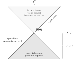
In the local continuum theory with the stated causal normalization, the first-order response is supported in the closed past light cone. Allowed contact terms are at its tip. Future insertions cancel between the forward and backward branches; the diagram is a schematic support statement.
The corresponding in–out correction is instead
This is the correct first variation of an in–out transition amplitude. It is not a causal expectation value, because it is not trying to be one.
Oscillator Green functions and state dependence
Section titled “Oscillator Green functions and state dependence”The same lesson can be seen without fields. Let be the mechanical mass and the oscillator frequency:
The ground-state Feynman function is
The cusp at supplies the delta function:
Fourier transforming gives
and the ground-state boundary condition selects
The differential equation alone does not fix the Green function. Because
one may add homogeneous on-shell pieces:
Their coefficients encode the state and boundary condition. The differential operator fixes the response away from its characteristic frequencies, but it cannot determine the population already present on shell.
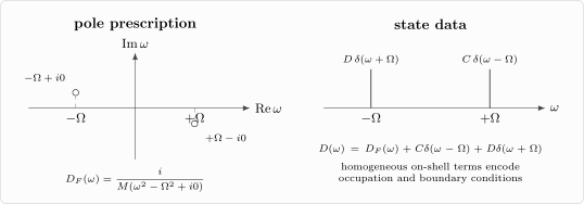
The equation fixes the off-shell part of the Green function but not the on-shell homogeneous terms. The pole prescription and the state determine which Green function is meant.
For a number eigenstate or a normalized diagonal density matrix with finite mean occupation,
one finds
and hence
The ground-state result is recovered at . A thermal state has
Thus a Green function is not merely the inverse of a differential operator. It is the inverse plus a boundary condition plus a state.
Time-dependent backgrounds and the road to pair creation
Section titled “Time-dependent backgrounds and the road to pair creation”The next page studies backgrounds that change in time. In oscillator language the mode equation becomes
with, for example,
A positive-frequency mode in the far past need not remain purely positive-frequency in the far future. This is the origin of Bogoliubov coefficients and particle creation:
The in–out propagator uses boundary data at both ends: for fixed second time it is negative-frequency as the first time tends to the far past and positive-frequency as that time tends to the far future. Equivalently, its two homogeneous solutions are selected by the in- and out-vacuum boundary conditions. The in–in propagators are instead fixed by an initial state and track what that state evolves into. For stable scattering in empty space, both languages coexist peacefully. For particle production, vacuum decay, transport, and horizons, the distinction becomes the calculation.
Summary
Section titled “Summary”The ordinary Feynman functional is an in–out object. It computes transition amplitudes and the in–out effective action. Its vacuum bubbles exponentiate into the vacuum persistence amplitude , and an imaginary part of signals loss of probability from the vacuum channel.
The Schwinger–Keldysh formalism is an in–in construction. It doubles fields, sources, vertices, and propagators because it evolves both the ket and the bra. For a normalized initial density matrix and unitary evolution, equal sources give . In the Keldysh rotation, differentiating with respect to the auxiliary source inserts an observable, whereas varying the common source produces its physical response.
The four real-time propagators are Feynman, anti-Feynman, and two Wightman functions. In the basis they become the statistical function , the retarded and advanced functions, and a vanishing entry. Causal response appears when the two contour branches combine time-ordered terms into commutators.
A Green function is not just an inverse operator. It also contains a pole prescription and state data. That fact is harmless in equilibrium, but indispensable in nonequilibrium QFT.
Common pitfalls
Section titled “Common pitfalls”Confusing Feynman propagation with causal response. The Feynman propagator is generally nonzero at spacelike separation. Causality is carried by commutators and retarded functions, not by the support of alone.
Calling an in–out matrix element an expectation value. A denominator-normalized Feynman expression still has a final-vacuum boundary condition. A detector reading at time is an in–in expectation value in the evolved initial state.
Dropping the minus-branch sign. The branch carries , so its vertices have conjugate signs. Without this sign, the two evolutions are not and , and vacuum-bubble cancellation fails.
Forgetting the initial density matrix. The contour defines an evolution problem only after is specified. Non-Gaussian initial correlations can add vertices at and cannot in general be reproduced by changing a free occupation number.
Using vacuum Wightman functions for a populated state. The displayed formulas are vacuum formulas. Thermal or occupied Gaussian states add occupation factors even though the free spectral support remains on shell.
Thinking the differential equation fixes the propagator. It fixes the off-shell inverse. The pole prescription and homogeneous on-shell terms encode boundary conditions and state data.
Exercises
Section titled “Exercises”Exercise 1: First-order causal response
Section titled “Exercise 1: First-order causal response”Derive the first-order in–in response formula
Solution
Use
and
Then
Keeping terms through first order gives
Thus
The upper limit and the commutator are the two ingredients that make the expression retarded.
Exercise 2: Contour identities
Section titled “Exercise 2: Contour identities”Starting from
where , prove
and
Solution
Adding the two definitions gives
Away from coincident times, , so
For the retarded combination,
This is
Similarly,
so both expressions agree.
Exercise 3: Occupied oscillator propagator
Section titled “Exercise 3: Occupied oscillator propagator”For and , take
and assume a normalized diagonal state with finite mean occupation,
Compute , , and the time-ordered propagator .
Solution
Multiplying the two oscillator expansions gives
Therefore
Interchanging and gives
The time-ordered function is
Combining the two cases yields
For , this reduces to the ground-state Feynman function.
Exercise 4: Closed-contour normalization
Section titled “Exercise 4: Closed-contour normalization”Show that the closed-time-path generating functional satisfies
for a normalized initial density matrix and a common real source generating unitary evolution, while the in–out vacuum functional need not have unit modulus.
Solution
By definition,
Set . Then
Using cyclicity of the trace,
Unitary time evolution gives , hence
The in–out functional is instead
This is a transition amplitude between specified boundary states. Its modulus can be smaller than one when other final states are available.
Exercise 5: Microcausality and response support
Section titled “Exercise 5: Microcausality and response support”Let
Use the fixed local composite normalization, causal extension and smooth switching/smearing prescription of the main text. Show that the first-order correction to is a retarded commutator integral, and explain why its support lies in the closed past light cone, including possible contact terms at the origin. No unrestricted adiabatic limit or finite value of the response is assumed.
Solution
Set
The first-order in–in response is
Substituting the interaction Hamiltonian gives
The time integrals denote the common causal extension, including its prescribed endpoint contact terms. Equivalently, with the kernel defined in the main text and the smooth test functions understood,
The prescribed local composites commute at spacelike separation. Therefore, away from coincidence,
The retarded extension has support in the closed past half-space; locality further restricts it to the closed past light cone. Local terms at the origin obey this support condition and are not discarded by the all-space pairing. Their coefficients belong to the chosen normalization, not to the microcausality argument.
Exercise 6: The Keldysh rotation
Section titled “Exercise 6: The Keldysh rotation”Use the definitions
and
to show that
Explain why equal physical sources correspond to . Then use the four contour propagators to show
Solution
Invert the definitions:
and
Then
The and terms cancel, leaving
Equal physical sources mean , so
The auxiliary source is nevertheless useful because differentiating with respect to it inserts the physical field before the physical limit is taken.
For the correlators,
where the contour identity was used in the second step. Similarly,
and
Finally,
Thus the basis separates the statistical, retarded, and advanced functions and makes the unitarity zero explicit.
References
Section titled “References”- Jürgen Berges, “Introduction to Nonequilibrium Quantum Field Theory,” AIP Conference Proceedings 739 (2005), 3–62. DOI: 10.1063/1.1843591. Open PDF: arXiv hep-ph/0409233v1, 20 September 2004. Page references above use this preprint’s printed pagination.
- Romeo Brunetti and Klaus Fredenhagen, “Microlocal Analysis and Interacting Quantum Field Theories: Renormalization on Physical Backgrounds,” Communications in Mathematical Physics 208 (2000), 623–661. DOI: 10.1007/s002200050004. Open PDF: arXiv math-ph/9903028v1, 12 March 1999. Page references above use this preprint’s printed pagination.
Further reading
Section titled “Further reading”- Esteban A. Calzetta and Bei-Lok B. Hu, Nonequilibrium Quantum Field Theory, Cambridge University Press, 2008.
- Richard P. Feynman and Frank L. Vernon Jr., “The Theory of a General Quantum System Interacting with a Linear Dissipative System,” Annals of Physics 24 (1963), 118–173.
- Alex Kamenev, Field Theory of Non-Equilibrium Systems, Cambridge University Press, 2011.
- Leonid V. Keldysh, “Diagram Technique for Nonequilibrium Processes,” Soviet Physics JETP 20 (1965), 1018–1026.
- Jørgen Rammer, Quantum Field Theory of Non-equilibrium States, Cambridge University Press, 2007.
- Julian Schwinger, “Brownian Motion of a Quantum Oscillator,” Journal of Mathematical Physics 2 (1961), 407–432.