Gaussian Fluctuations and Effective Free Energy

The quadratic fluctuation operator around a stationary configuration determines the leading covariance, linear stability, and one-loop contribution to the free energy. Positive nonzero eigenvalues give ordinary Gaussian modes; exact zero modes require collective coordinates; a negative mode means the configuration is not a stable equilibrium saddle. The approximation fails when infrared fluctuations, multiple saddles, or interactions among fluctuation modes are no longer perturbative.

The determinant expansion and its negative- and zero-mode qualifications are developed in Kleinert 2009, chs. 2 and 5.

Required background. Correlations, Susceptibilities, and Correlation Lengths fixes the static covariance and screening language. Gaussian Fields and Sources supplies functional Gaussian integration. Helpful background. Zero Modes, Collective Coordinates, and Moduli Measures develops the non-Gaussian treatment of symmetry directions.

Expansion about an equilibrium background

Let $\mathcal F[\phi]$ be a regulated coarse-grained free-energy functional and $\bar\phi$ a stationary configuration,

$$\left.\frac{\delta\mathcal F}{\delta\phi(x)}\right|_{\bar\phi}=0.$$

Writing $\phi=\bar\phi+\eta$ gives

$$\mathcal F[\bar\phi+\eta] =\mathcal F[\bar\phi] +\frac12\int\mathrm d^{d-1}x\,\mathrm d^{d-1}y\, \eta(x)\mathcal K(x,y)\eta(y) +\mathcal F_{\mathrm{int}}[\eta],$$

where

$$\mathcal K(x,y)= \left.\frac{\delta^2\mathcal F} {\delta\phi(x)\delta\phi(y)}\right|_{\bar\phi}.$$

At Gaussian order the covariance is

$$\langle\eta(x)\eta(y)\rangle_G=T\,\mathcal K^{-1}(x,y)$$

on the subspace where the inverse exists. The factor of $T$ follows because the statistical weight is $e^{-\mathcal F/T}$. If the displayed functional is already the dimensionless Euclidean action $S_E=\mathcal F/T$, that factor is absent. This simple translation prevents a common normalization error.

Determinants and the one-loop free energy

Diagonalize the regulated Hessian, $\mathcal K u_n=\lambda_nu_n$. For positive eigenvalues,

$$Z_G=e^{-\mathcal F[\bar\phi]/T} \prod_n\left(\frac{2\pi T}{\lambda_n}\right)^{1/2},$$

and therefore

$$\mathcal F_{\mathrm{eff}}^{(1)}[\bar\phi] =\mathcal F[\bar\phi] +\frac{T}{2}\operatorname{Tr}'\log\mathcal K +\text{measure and counterterm terms}.$$

The prime omits exact zero modes. The determinant is regulator dependent and cannot be quoted without its subtraction prescription. In a QFT application the ultraviolet divergence is removed by the counterterms of the underlying theory or matched EFT; temperature does not license a new arbitrary subtraction.

For a homogeneous scalar background with

$$\mathcal F=\int\mathrm d^{d-1}x \left[\frac12(\nabla\phi)^2+U(\phi)\right],$$

one has $\mathcal K=-\nabla^2+U''(\bar\phi)$. The one-loop density is formally

$$\Delta f_1 =\frac{T}{2}\int\frac{\mathrm d^{d-1}k}{(2\pi)^{d-1}} \log\!\left(\mathbf k^2+M^2\right), \qquad M^2=U''(\bar\phi).$$

Differentiating with respect to $M^2$ turns the logarithm into the checked covariance integral. Integrating back requires a renormalization condition; discarding the integration constant without stating it can change pressure comparisons.

Zero and negative directions

If a continuous symmetry moves the saddle without changing $\mathcal F$, $\mathcal K$ has a zero eigenvector. The Gaussian integral over that coordinate diverges because a quadratic coordinate is being used along a flat orbit. Replace it by a collective coordinate $a$ and its Jacobian,

$$\int\mathcal D\eta \longrightarrow J_{\mathrm{coll}}\int\mathrm da\, \int\mathcal D\eta_{\perp}.$$

The group or moduli-space volume is physical only after gauge redundancies are divided out and global symmetries are treated with the appropriate finite-volume normalization.

A negative eigenvalue makes the real Gaussian integral divergent. For a coarse-grained free-energy landscape it indicates local instability. For a metastable bounce, one negative mode instead participates in extracting an imaginary part and a decay rate; that specialized contour and prefactor analysis belongs to Bounces, Determinants, and Thermal Nucleation Rates. A negative direction must never be silently replaced by an absolute determinant on an equilibrium page.

When Gaussian control fails

For a scalar theory near criticality, compare the fluctuation of a coarse-grained field over a correlation volume with the squared mean-field order parameter. Parametrically,

$$\langle(\delta\phi)^2\rangle_{\xi} \sim T\int^{\xi^{-1}} \frac{\mathrm d^{d-1}k}{(2\pi)^{d-1}} \frac1{k^2+\xi^{-2}}.$$

The Ginzburg criterion demands this be small compared with the scale on which the quartic interaction changes the saddle. When it fails, loop counting is reorganized by critical scaling; adding one more determinant term does not restore control.

Other failure signals are a small Hessian gap, extensive degeneracy, a determinant dominated by regulator modes, competing saddles with comparable weight, or a loop correction as large as the tree-level difference being interpreted.

Independent checks

• Differentiate $\frac{T}{2}\operatorname{Tr}\log\mathcal K$ and recover $\frac{T}{2}\operatorname{Tr}(\mathcal K^{-1}\delta\mathcal K)$.
• Verify dimensions: an eigenvalue of $-\nabla^2+M^2$ has mass dimension two, so the determinant needs a reference scale.
• Count zero modes from broken continuous symmetries and compare with the collective-coordinate dimension.
• Confirm that all retained nonzero eigenvalues are positive for a claimed stable phase.
• Vary regulator and subtraction while holding the matched long-distance observables fixed.

The schematic below organizes the relationships used on this page. Inspect it with this question in mind: How do Euclidean configurations, correlations, Gaussian fluctuations, phases, and thermodynamic limits relate?

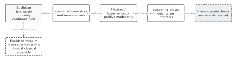
A Euclidean weight defines correlations; a positive Hessian licenses Gaussian fluctuations locally, while phase coexistence and spontaneous breaking require a separately ordered thermodynamic and source limit. Solid connections show the primary relation; dashed outlines or arrows mark qualifications and failure boundaries. The diagram is schematic and not to scale.

The surrounding discussion supplies the relevant equations and checks in text form; the figure is a navigational summary.

Exercise

For $\mathcal K=-\partial_x^2+m^2$ on a periodic interval, what happens to the constant mode as $m^2\to0^+$?

Solution

The eigenvalues are $(2\pi n/L)^2+m^2$. The $n=0$ covariance is $T/m^2$ and its determinant contribution is $(T/2)\log m^2$, so the Gaussian fluctuation diverges as $m^2\to0^+$. At $m=0$ the constant direction must be controlled by an interaction, a constraint, or a collective-coordinate treatment; the inverse Hessian does not exist on the full space.

References

• Coleman, Sidney. “The Uses of Instantons.” In Aspects of Symmetry, 265–350. Cambridge: Cambridge University Press, 1985. doi:10.1017/CBO9780511565045.008.
• Kleinert, Hagen. Path Integrals in Quantum Mechanics, Statistics, Polymer Physics, and Financial Markets. 5th ed. Singapore: World Scientific, 2009. doi:10.1142/7305.
• Zinn-Justin, Jean. Quantum Field Theory and Critical Phenomena. 5th ed. Oxford: Oxford University Press, 2021. doi:10.1093/oso/9780198834625.001.0001.