Transport Extraction, Inverse Problems, and Error Budgets

A dataset identifies only those transport combinations that survive the smoothing of its forward kernel, its correlated errors, and defensible variations of priors and model discrepancy. Euclidean thermal data often constrain broad spectral averages far better than a pointwise dc slope. A publication-quality extraction must therefore propagate covariance, display resolution, pass synthetic recovery, vary the spectral model, and match its conclusion to what is identifiable: a value, a broad interval, a moment, or only compatibility with a family.

Required background. Spectral functions and transport peaks distinguishes the structures an inference might seek. Spectral reconstruction as an inverse problem derives the thermal kernel and analytic-continuation ambiguity. Helpful background. Multistage Bayesian global inference and evidence develops correlated forward-model inference in a more elaborate setting.

The forward map determines identifiability

With $\rho=-2\operatorname{Im}G_R$, a bosonic Euclidean correlator has the representation

$$G_E(\tau)=\int_0^\infty\frac{d\omega}{2\pi}\, \rho(\omega) \frac{\cosh[\omega(\beta/2-\tau)]} {\sinh(\beta\omega/2)}, \qquad 0<\tau<\beta.$$

At small frequency the kernel behaves as $2T/\omega+O(\omega)$, so many different low-frequency shapes with the same weighted area produce nearly identical Euclidean data. The derivative $\rho'(0)$ defining a viscosity or conductivity can therefore be poorly determined even when $G_E$ is measured precisely.

After discretization and subtraction of known contacts or ultraviolet pieces,

$$\mathbf y=\mathbf K\boldsymbol\rho+\boldsymbol\epsilon, \qquad \langle\boldsymbol\epsilon\boldsymbol\epsilon^T\rangle=\mathbf C_{\mathrm{data}}.$$

The singular values of the whitened matrix $\mathbf C_{\mathrm{data}}^{-1/2}\mathbf K$ usually decay rapidly. Directions in spectral space associated with small singular values are unidentifiable without added information. Reducing pointwise error bars cannot recover a direction that the kernel nearly annihilates.

Covariance is part of the likelihood

Thermal correlator samples at different Euclidean times, momenta, temperatures, or lattice spacings are correlated. Replacing $\mathbf C_{\mathrm{data}}$ by its diagonal changes which residuals are penalized and can create artificial precision. A usable covariance estimate must report its sampling procedure, conditioning or shrinkage, retained eigenmodes, and uncertainty.

Model discrepancy belongs in the forward distribution rather than being appended as an informal percentage. Schematically,

$$\mathbf C_{\mathrm{tot}} =\mathbf C_{\mathrm{data}} +\mathbf C_{\mathrm{disc}} +\mathbf C_{\mathrm{emul}} +\mathbf C_{\mathrm{model}},$$

with correlations retained. Discretization, finite volume, interpolation, emulator error, normalization, and contact subtraction may instead be represented by nuisance parameters in a joint hierarchy. The choice depends on what can be calibrated, but no material term should disappear from the likelihood.

Priors regularize rather than reveal information

In a finite-dimensional linear Gaussian example with prior

$$\boldsymbol\rho\sim \mathcal N(\mathbf m,\mathbf S),$$

the posterior covariance and mean are

$$\begin{aligned} \boldsymbol\Sigma_{\mathrm{post}} &=\left( \mathbf K^T\mathbf C_{\mathrm{tot}}^{-1}\mathbf K +\mathbf S^{-1} \right)^{-1},\\ \boldsymbol\mu_{\mathrm{post}} &=\boldsymbol\Sigma_{\mathrm{post}} \left( \mathbf K^T\mathbf C_{\mathrm{tot}}^{-1}\mathbf y +\mathbf S^{-1}\mathbf m \right). \end{aligned}$$

Along weakly constrained directions, the posterior approaches the prior. Positivity, smoothness, asymptotic tails, and sum rules can be justified prior information, but their strength and possible violation must be varied. Comparing only two implementations of the same restrictive ansatz is not a meaningful robustness test.

Nonlinear peak models require sampling rather than these closed formulas, and multimodality or parameter degeneracy must be shown rather than compressed into a symmetric error bar. A narrow transport peak can trade height against width while leaving its area fixed; the posterior may identify the area but not either parameter separately.

Resolution and claim-level observables

For the Gaussian linear problem, the response of the posterior mean to a change in the true spectrum is described by

$$\mathbf R =\boldsymbol\Sigma_{\mathrm{post}} \mathbf K^T\mathbf C_{\mathrm{tot}}^{-1}\mathbf K.$$

Each row is an averaging kernel. A broad row means that a nominal “value at $\omega_0$” is actually a weighted average over a wide interval. Backus–Gilbert methods make this tradeoff explicit by constructing a minimum-width averaging kernel at controlled variance Backus and Gilbert 1968, §§2–4.

Modern lattice formulations make the averaging-kernel target and regularization explicit Hansen, Lupo, and Tantalo 2019, §§2–4, Open PDF, while transport applications illustrate why a good Euclidean fit need not resolve the dc slope Meyer 2011, §§3–4, Open PDF.

Report the observable that the resolution supports. Useful levels are:

• a point estimate and interval for a coefficient only when the low-frequency slope is resolved across model variations;
• a broad interval when the sign or scale is stable but the detailed peak is not;
• a spectral integral or smeared value when only an averaging-kernel combination is data dominated;
• an upper or lower bound when positivity and exact moments license one;
• compatibility with a family when even those combinations remain prior sensitive.

The transport-extraction covariance reference provides the common record for operator conventions, contacts, limits, priors, covariance, resolution, windows, regulator and volume limits, cross-checks, and input date.

Synthetic recovery and adversarial checks

Before applying an inference to precious data, generate mock observations through the same forward kernel and covariance. Include spectra inside the inference family and adversarial spectra outside it: an unresolved narrow peak, two nearby rates, a long-time-tail cusp, shifted ultraviolet weight satisfying the same sum rule, and no transport peak. Hide the truth during fitting when practical.

Recovery must be judged at the claim level. If the method cannot distinguish a one-peak truth from a two-scale truth but recovers their common integral, it is validated for that integral, not for the peak width. Posterior predictive agreement with the input correlator is necessary but not sufficient because an ill-conditioned kernel maps many spectra to the same data.

Vary fit windows, temporal points, covariance conditioning, continuum forms, volumes, ultraviolet matching scales, priors, and discrepancy models. Withhold some data or observables for validation. Compare against exact sum rules, Ward identities, thermodynamic susceptibilities, and—in a controlled benchmark—real-time or kinetic results.

A complete error budget

Separate at least the following contributions when they are relevant:

1. statistical sampling and covariance estimation;
2. source normalization, contacts, and magnetization subtraction;
3. finite volume, cutoff, and continuum extrapolation;
4. Euclidean-to-real-time resolution and continuation prior;
5. spectral ansatz and omitted structures;
6. ultraviolet matching and sum-rule uncertainty;
7. emulator, interpolation, or solver error;
8. parameter degeneracy and model discrepancy;
9. validation coverage and evidence cutoff.

Do not add correlated terms in quadrature without justification. Publish the joint posterior or covariance for derived transport combinations when possible. A comparison across methods is meaningful only after operator normalization, source convention, contacts, and limit order have been reconciled.

Evidence boundary

This page describes inference methodology checked against the cited literature through 10 August 2026. It reports no numerical transport coefficient and does not elevate any particular continuation prior or spectral ansatz to a universally preferred method. Current reviews emphasize that reliable conclusions depend on observable-specific resolution and validation rather than a method label Rothkopf 2022, §§2–5.

The final two boxes and the downward branch visualize this page’s decision rule. Inspect how data, covariance, priors, and resolution enter inverse inference before a coefficient or combination is reported; a broad or unresolved result terminates in non-identification instead.

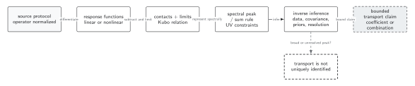
Inverse inference converts the fully specified forward problem and correlated dataset into a claim whose strength is limited by resolution and model discrepancy. A resolved slope may support a coefficient; weaker information may support only an interval, moment, bound, or compatibility class. The downward branch is the scientifically correct outcome when no transport combination is uniquely identified. The diagram is schematic.

In text: whiten by the full covariance, inspect singular directions or averaging kernels, vary priors and discrepancy models, pass synthetic and withheld-data tests, and propagate regulator and volume limits. Report only the combination that remains data-sensitive across those checks.

Exercise: a prior-dominated direction

Let $\mathbf v$ be a normalized spectral direction with $\mathbf K\mathbf v=0$. In the Gaussian model, show that data cannot update the prior variance or mean component along $\mathbf v$.

Solution

Because $\mathbf K\mathbf v=0$,

$$\mathbf v^T\mathbf K^T\mathbf C_{\mathrm{tot}}^{-1}\mathbf K\mathbf v=0, \qquad \mathbf v^T\mathbf K^T\mathbf C_{\mathrm{tot}}^{-1}\mathbf y=0.$$

If $\mathbf v$ is also a prior eigenvector with variance $s_v$, the posterior precision in that direction is only $s_v^{-1}$ and the posterior mean component remains $\mathbf v^T\mathbf m$. More generally, prior correlations can mix $\mathbf v$ with identifiable directions, but any update then comes from the prior structure, not direct likelihood sensitivity to $\mathbf v$. Reporting that component as data determined would be false.

References

• Backus, George, and Freeman Gilbert. 1968. “The Resolving Power of Gross Earth Data.” Geophysical Journal of the Royal Astronomical Society 16 (2): 169–205. DOI.
• Hansen, Martin, Alessandro Lupo, and Nazario Tantalo. 2019. “Extraction of Spectral Densities from Lattice Correlators.” Physical Review D 99 (9): 094508. DOI. Open PDF.
• Meyer, Harvey B. 2011. “Transport Properties of the Quark–Gluon Plasma: A Lattice QCD Perspective.” European Physical Journal A 47: 86. DOI. Open PDF.
• Rothkopf, Alexander. 2022. “Inverse Problems, Real-Time Dynamics and Lattice Simulations.” Frontiers in Physics 10: 1028995. DOI. Open PDF.

The chapter closes here. Return to Sources, Linear Response, and Kubo Formulae to verify that any inferred quantity matches the original operator and source definition, or to Transport Sum Rules and Ultraviolet Constraints to test its integrated weight.