Thermal Loop Expansions and Scale Power Counting

Thermal perturbation theory must be counted by momentum, frequency, occupation, and observable before diagrams are evaluated. Hard modes carry momenta of order $T$; bosonic zero modes can live at soft screening scales such as $\sqrt{\lambda}T$ in scalar theory or $gT$ in gauge theory; non-Abelian magnetic modes remain at $g^2T$. Bose enhancement $n_B(k)\sim T/k$ promotes soft loops, so one vacuum loop factor cannot be used uniformly across these regimes.

The hard/soft separation and effective-theory counting of high-temperature thermodynamics are demonstrated by Braaten and Nieto 1995, §§ II–III, pp. 6992–6999.

Required background. Imaginary Time and Matsubara Frequencies supplies zero modes and thermal sums. Power Counting of Divergences and Perturbative Renormalizability supplies ultraviolet counting. Helpful background. Scale Separation, Locality, and the Domain of an EFT gives the EFT interpretation.

Inventory the scales first

A calculation should list at least

$$T,\quad m,\quad \lvert\mathbf p_{\mathrm{ext}}\rvert,\quad \omega_{\mathrm{ext}},\quad \mu,\quad \Gamma,\quad \Lambda_{\mathrm{UV}},$$

and any dynamically generated screening scale. It should also identify whether the observable is static, lightlike, timelike, or hydrodynamic. The same self-energy has different expansions at $(\omega=0,\mathbf p\to0)$ and $(\omega\sim\lvert\mathbf p\rvert\sim T)$.

For weakly coupled massless $\lambda\phi^4/4!$ theory in four dimensions,

$$m_{\mathrm{th}}^2\sim\lambda T^2, \qquad m_{\mathrm{th}}\sim\sqrt{\lambda}T.$$

For a hot non-Abelian gauge theory,

$$T\gg gT\gg g^2T$$

at asymptotically weak coupling. These labels are parametric. Numerical separation can be poor unless $g\ll1$, and different observables begin to feel the scales at different orders.

Bose enhancement changes loop counting

For $k\ll T$,

$$n_B(k)=\frac1{e^{k/T}-1}\simeq\frac{T}{k}.$$

A soft bosonic propagator and loop measure therefore contribute schematically

$$T\int\frac{\mathrm d^3k}{(2\pi)^3} \frac1{k^2+m_s^2} \sim Tm_s,$$

not the hard $T^2$ scaling inferred by setting all momenta to $T$. In scalar theory, an extra zero-mode insertion in a ring scales as

$$\lambda T\int\frac{\mathrm d^3k}{(2\pi)^3} \frac1{(k^2+m_s^2)^2} \sim\frac{\lambda T}{m_s}.$$

With $m_s\sim\sqrt\lambda T$, this is $O(\sqrt\lambda)$ rather than $O(\lambda)$. An infinite family produces nonanalytic powers such as $\lambda^{3/2}$ in thermodynamic quantities. Fermions have no zero Matsubara mode and no analogous static Bose enhancement, though soft gauge exchange can still make fermionic observables infrared sensitive.

Observable-dependent countings

Regime	External kinematics	Relevant reorganization	Early failure signal
hard thermodynamics	loop momenta $\sim T$	ordinary thermal loop expansion plus vacuum renormalization	residual soft contribution at the same order
static screening	$\omega=0$, $p\sim gT$ or $\sqrt\lambda T$	screened propagators or dimensionally reduced EFT	expansion in $\Pi/p^2$ is not small
real-time soft gauge response	$\omega,p\sim gT$	hard-thermal-loop effective theory	gauge-dependent or nonlocal result from fixed order
transport/lightlike rate	$\omega,p$ near a cut or collinear shell	kinetic and ladder/LPM resummation	pinching poles or formation time comparable to collision time
critical region	$\xi^{-1}\ll T$	dynamic/static critical EFT and RG	Ginzburg criterion fails
non-Abelian magnetostatic sector	$p\sim g^2T$	nonperturbative three-dimensional input	every additional magnetic loop is unsuppressed

The coupling symbol alone cannot choose a row.

A pre-diagram workflow

1. Declare state, observable, external kinematics, and desired accuracy.
2. List hard, soft, ultrasoft, mass, width, and frequency scales.
3. Expand occupation factors in each momentum region rather than globally.
4. Determine whether propagator corrections are small in that region.
5. Identify zero modes, pinching pairs, collinear denominators, and gauge sectors.
6. Match overlapping regions so no scale is counted twice.
7. State the first omitted term and the condition under which it is smaller.

The schematic below organizes the relationships used on this page. Inspect it with this question in mind: How does a thermal loop calculation pass from scale counting to a physical observable?

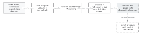
Thermal power counting chooses hard and soft regions; sum-integrals are split into vacuum and thermal parts, vacuum counterterms renormalize them, and mass, width, infrared, RG, and gauge checks bound the final observable. Solid connections show the primary relation; dashed outlines or arrows mark qualifications and failure boundaries. The diagram is schematic and not to scale.

The surrounding discussion supplies the relevant equations and checks in text form; the figure is a navigational summary.

Exercise

Why is expanding $(k^2+m_s^2)^{-1}=k^{-2}-m_s^2k^{-4}+\cdots$ invalid throughout a zero-mode integral?

Solution

The expansion requires $m_s^2/k^2\ll1$, but the integral includes $k\lesssim m_s$, where every term is as large as the previous and increasingly infrared divergent. Keeping $m_s$ in the soft propagator resums precisely the region in which the Taylor series is nonuniform.

References

• Braaten, Eric, and Agustín Nieto. “Effective Field Theory Approach to High Temperature Thermodynamics.” Physical Review D 51, no. 12 (1995): 6990–7006. doi:10.1103/PhysRevD.51.6990.
• Linde, A. D. “Infrared Problem in Thermodynamics of the Yang–Mills Gas.” Physics Letters B 96, nos. 3–4 (1980): 289–292. doi:10.1016/0370-2693(80)90769-8.
• Parwani, Rajesh R. “Resummation in a Hot Scalar Field Theory.” Physical Review D 45, no. 12 (1992): 4695–4705. doi:10.1103/PhysRevD.45.4695.