

Noisy Spectral Reconstruction as an Inverse Problem
A supplied Euclidean reconstruction licenses a real-time claim only after its thermal channel is identified and its feature survives KMS, adjoint, positivity-domain, contact, ultraviolet, sum-rule, finite-volume, resolution, covariance, and order-of-limits tests. A narrow reconstructed curve may support only a smeared spectral integral; a transport coefficient requires resolved low-frequency behavior in the correct zero-frequency and zero-momentum order. Thermal constraints reduce the admissible set but rarely make a finite noisy inverse unique.
The Bayesian inverse formulation and resolution dependence used here are reviewed by Jarrell and Gubernatis 1996, §§ 3–5, pp. 145–177.
Required background. Exact Euclidean–Real-Time Analytic Continuation distinguishes exact uniqueness from numerical stability. Spectral Reconstruction and Ill-Posed Euclidean Inverse Problems develops the reconstruction algorithms, resolution functions, priors, and covariance machinery.
Conditions for a thermal interpretation
Section titled “Conditions for a thermal interpretation”A spectral reconstruction must supply at least
Here is the resolution or influence kernel. Volume 11 then adds the physics fields that determine what means:
| Field | Required question | Claim blocked if absent |
|---|---|---|
| Operator and adjoint | Is the channel Hermitian, charged, mixed, or gauge variant? | positivity and detailed-balance statements |
| State | Which , chemical potentials, phase, volume, and boundary conditions? | KMS and equilibrium interpretation |
| Spectral convention | What commutator or anticommutator and normalization define ? | comparison with sum rules or other methods |
| Contacts/subtractions | Which polynomial and zero-mode terms are separated? | static and ultraviolet inference |
| Limit order | Is taken before or after , , and ? | transport or susceptibility claim |
| Resolution/covariance | Which spectral averages are data identified? | pointwise peak, width, or coefficient |
These specifications fix the physical observable; changing any one can change the quantity being reconstructed.
Classifying a low-frequency feature
Section titled “Classifying a low-frequency feature”Suppose a bosonic channel is reconstructed near . The Euclidean kernel behaves as
Euclidean data are therefore sensitive mainly to an integral of , not to the detailed shape of a narrow transport peak. Several spectra with different widths and slopes can have nearly identical Euclidean correlators.
Use three claim levels:
- Resolved integral: a declared weighted spectral average is stable under resolution and prior variations.
- Conditional feature: a peak or width is obtained only within a model family and is reported with that family and negative controls.
- Transport coefficient: the required slope or limit, such as , is resolved after contact terms, momentum limits, continuum extrapolation, and covariance are controlled.
If only level 1 passes, reporting level 3 is an overclaim.
Constraint tests
Section titled “Constraint tests”KMS and oddness. Reconstruct one independent spectral object and generate its positive- and negative-frequency partners using the declared detailed-balance relation. Fitting them independently can violate equilibrium.
Qualified positivity. Apply only to a Hermitian positive-metric channel. For a matrix channel, test positive semidefiniteness of integrated quadratic forms.
Sum rules. Evaluate each rule after applying the reconstruction’s resolution kernel to the same target or after propagating ultraviolet tail uncertainty. A truncated frequency window cannot be assigned the missing moment without a tail model.
Forward closure. Push every candidate spectrum through the exact Euclidean kernel and full covariance. Good closure is necessary but not sufficient because approximate null directions remain.
Adversarial alternatives. Construct a broad shoulder and a narrow peak whose Euclidean predictions differ by less than the correlated error. If the analysis selects one, identify whether the selection comes from data, positivity, a sum rule, or a prior.
Error budget and stopping rule
Section titled “Error budget and stopping rule”Separate statistical covariance, temporal discretization, spatial volume, continuum extrapolation, operator renormalization, contact subtraction, ultraviolet completion, reconstruction regularization, prior/model choice, frequency truncation, and momentum-limit order. Varying only the regularization parameter does not cover the other terms.
Stop at the strongest claim that passes all of the following:
- coverage on mock spectra outside the inference prior;
- stable resolved averages under scientifically plausible alternatives;
- correct KMS, sum-rule, and ultraviolet behavior;
- continuum and volume trends for the derived quantity;
- full-covariance forward residuals and held-out Euclidean data;
- an identifiability test against adversarial spectra; and
- a statement of which assumptions, rather than data, determine any remaining shape.
A KMS and spectral-continuation benchmark should execute this workflow on synthetic data with declared noise, regularization, and acceptance criteria.
The schematic below organizes the relationships used on this page. Inspect it with this question in mind: What connects thermal correlators, spectral densities, exact continuation, and finite-data reconstruction?
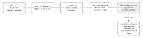
KMS and the commutator determine compatible Euclidean and retarded representations; exact analytic continuation is unique under its hypotheses, whereas reconstructing a spectrum from finite noisy data is an ill-posed inference problem. Solid connections show the primary relation; dashed outlines or arrows mark qualifications and failure boundaries. The diagram is schematic and not to scale.
The surrounding discussion supplies the relevant equations and checks in text form; the figure is a navigational summary.
Exercise
Section titled “Exercise”Two positive spectra have the same but transport peaks of widths and , with both widths far below the Euclidean resolution. What can the data identify?
Solution
They can identify the resolved weighted integral, subject to covariance and ultraviolet separation. They cannot distinguish the two widths or their different slopes. A quoted transport coefficient would therefore be conditional on the assumed peak shape or width prior.
References
Section titled “References”- Backus, George, and Freeman Gilbert. “The Resolving Power of Gross Earth Data.” Geophysical Journal of the Royal Astronomical Society 16, no. 2 (1968): 169–205. doi:10.1111/j.1365-246X.1968.tb00216.x.
- Jarrell, Mark, and J. E. Gubernatis. “Bayesian Inference and the Analytic Continuation of Imaginary-Time Quantum Monte Carlo Data.” Physics Reports 269, no. 3 (1996): 133–195. doi:10.1016/0370-1573(95)00074-7.
- Meyer, Harvey B. “Transport Properties of the Quark–Gluon Plasma: A Lattice QCD Perspective.” European Physical Journal A 47 (2011): 86. doi:10.1140/epja/i2011-11086-3; Open PDF.