Damping Rates, Thermal Cuts, and Quasiparticle Widths

The imaginary part of a retarded self-energy measures the loss and gain channels available to an excitation. Thermal cuts add stimulated emission, Pauli blocking, absorption, and scattering with medium constituents; KMS relates forward and reverse processes. A quasiparticle width follows only for an isolated narrow pole. Soft exchange, pinching denominators, and nearly collinear formation can promote entire ladder families, so a fixed-order cut may not be a leading-order rate.

The thermal cutting rules and statistical weights entering widths are derived by Weldon 1983, §§ II–IV, pp. 2008–2013.

Required background. Thermal Self-Energies and Mass Definitions fixes the pole and width. Cutkosky Cutting Rules supplies vacuum discontinuities. Helpful background. Soft and Collinear Singularities diagnoses enhancements; Gauge-Theory Effective Kinetic Theory owns the leading-order gauge-plasma reorganization.

Width from the retarded pole

For inverse propagator

$$G_R^{-1}=\omega^2-E_{\mathbf p}^2-\Pi_R(\omega,\mathbf p),$$

write the pole as $\omega_*=\Omega_{\mathbf p}-i\Gamma_{\mathbf p}$. If $\Gamma\ll\Omega$ and the pole is isolated,

$$\Gamma_{\mathbf p} =-\frac{\operatorname{Im}\Pi_R(\Omega_{\mathbf p},\mathbf p)} {2\Omega_{\mathbf p}- \partial_\omega\operatorname{Re}\Pi_R(\Omega_{\mathbf p},\mathbf p)}.$$

For a stable retarded excitation, the pole lies in the lower half-plane and the numerator gives $\Gamma>0$ in this sign convention. A large $\Gamma/\Omega$ invalidates the quasiparticle expansion; one should report the full spectral response instead of a “lifetime.”

With $\omega_*=\Omega-i\Gamma$, $\Gamma$ is the pole damping rate. The full Breit–Wigner energy width is $2\Gamma$ in the narrow-resonance convention; sources that place $-i\Gamma/2$ in the pole call that full width $\Gamma$ instead.

Thermal cuts and statistical factors

Real-time cutting rules put internal lines on shell and sum over assignments corresponding to emission, absorption, and scattering. A bosonic final-state line contributes $1+n_B$, an occupied bosonic initial line contributes $n_B$; fermions give $1-n_F$ and $n_F$. For a schematic $1\leftrightarrow2$ process,

$$\Gamma_{1\to23}\propto \int\mathrm d\Pi_2\mathrm d\Pi_3 \lvert\mathcal M\rvert^2 \left[(1\pm f_2)(1\pm f_3)-f_2f_3\right] \delta^{(d)}(p_1-p_2-p_3),$$

where the relative signs and gain/loss organization depend on species and on whether a damping or production rate is being computed. KMS ensures that the collision term vanishes for equilibrium distributions.

The discontinuity includes vacuum thresholds and additional thermal support. Scattering off medium particles can create a Landau cut in spacelike kinematics, often $\lvert\omega\rvert<p$ for a simple isotropic plasma. This cut is not a new particle pole.

Inclusive rates and unstable external states

A production rate is usually tied to the spectral function of the operator coupling to the emitted probe. A damping rate refers to a pole of a medium excitation. They can involve the same self-energy discontinuity but different normalizations, external states, and detailed-balance factors.

An unstable particle is not an exact asymptotic state. Evaluating $\operatorname{Im}\Pi$ at a real tree-level shell is justified only within a narrow-width expansion. Gauge independence often requires evaluating a consistently defined complex pole and including all diagrams of the same reorganized order.

When fixed-order cutting fails

Soft exchange. A massless $t$-channel propagator produces infrared enhancement. Screening or HTL propagators must be used, with overlap subtractions.

Pinching poles. Products of retarded and advanced propagators near the same shell scale as an inverse width. Ladder diagrams can all contribute at the same order, as in transport coefficients.

Collinear formation. Nearly collinear emission can form over a time comparable with the mean free time. Multiple soft scatterings interfere—the Landau–Pomeranchuk–Migdal effect—and a single cut is insufficient.

Gauge cancellation. A subset of self-energy diagrams can be gauge dependent. Ward identities and the complete leading set are part of the rate.

Rate consistency checks

1. Declare whether the result is a pole width, inclusive rate, or kinetic relaxation eigenvalue.
2. Fix the retarded sign, cut orientation, external normalization, and state.
3. Verify KMS/detailed balance at equilibrium.
4. Include vacuum and thermal discontinuities without double counting.
5. Test soft, collinear, and pinching power counting.
6. Check gauge identities and the complex-pole or operator definition.
7. Stop at a full spectral function if the pole is broad.

The schematic below organizes the relationships used on this page. Inspect it with this question in mind: How does a thermal loop calculation pass from scale counting to a physical observable?

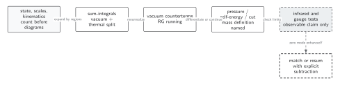
Thermal power counting chooses hard and soft regions; sum-integrals are split into vacuum and thermal parts, vacuum counterterms renormalize them, and mass, width, infrared, RG, and gauge checks bound the final observable. Solid connections show the primary relation; dashed outlines or arrows mark qualifications and failure boundaries. The diagram is schematic and not to scale.

The surrounding discussion supplies the relevant equations and checks in text form; the figure is a navigational summary.

Exercise

Why does the factor $1+n_B(E)$ not by itself represent a thermal production rate?

Solution

$1+n_B$ is only stimulated emission for one bosonic final line. A physical rate also requires matrix elements, phase space, all initial distributions, Pauli or Bose factors for other lines, inverse processes, normalization, and the correct cut. In equilibrium, gain and loss combine according to KMS; retaining one factor alone generally violates detailed balance.

References

• Kobes, Randy L., and Gordon W. Semenoff. “Discontinuities of Green Functions in Field Theory at Finite Temperature and Density.” Nuclear Physics B 260, no. 3–4 (1985): 714–746. doi:10.1016/0550-3213(85)90056-2.
• Weldon, H. Arthur. “Simple Rules for Discontinuities in Finite-Temperature Field Theory.” Physical Review D 28, no. 8 (1983): 2007–2015. doi:10.1103/PhysRevD.28.2007.