Bosonic Zero Modes and Infrared Breakdown

Bosonic zero Matsubara modes behave as a lower-dimensional classical field and receive no frequency gap from the thermal circle. When their screening scale becomes comparable with loop self-energies, expanding around a massless propagator is nonuniform and infinitely many ring diagrams contribute at the same nominal accuracy. Scalar and electric gauge sectors can be screened and reorganized; the non-Abelian magnetostatic sector at $g^2T$ remains intrinsically nonperturbative.

The non-Abelian magnetostatic obstruction and its parametric order were identified by Linde 1980, pp. 289–292.

Required background. Thermal Loop Expansions and Scale Power Counting supplies the scale inventory. Thermal Self-Energies and Mass Definitions supplies screening. Helpful background. Screening and Infrared Scale Separation constructs the next effective description.

Scalar ring enhancement

Separate the bosonic zero mode in a static self-energy insertion. A ring with $N$ insertions contains the schematic factor

$$T\int\frac{\mathrm d^3k}{(2\pi)^3} \frac1{k^2} \left(\frac{\Pi(0,k)}{k^2}\right)^N.$$

For hard momenta, $\Pi/k^2\sim\lambda$ is small. For $k^2\sim\Pi\sim\lambda T^2$, every power is $O(1)$. Expanding the denominator has failed exactly in the region contributing the soft correction.

Keeping $m_s^2=\Pi(0,0)$ in the zero-mode propagator sums the geometric series. The ring contribution to the free energy contains

$$\Delta f_{\mathrm{ring}} =\frac{T}{2}\int\frac{\mathrm d^3k}{(2\pi)^3} \left[ \log\left(1+\frac{m_s^2}{k^2}\right) -\frac{m_s^2}{k^2} \right] \sim-Tm_s^3.$$

Since $m_s\sim\sqrt\lambda T$, this is $O(\lambda^{3/2}T^4)$. The subtraction removes the term already counted at fixed order. Omitting it double counts the one-insertion diagram.

Critical and dimensional dependence

Near a critical point the physical screening mass tends to zero, and the static scalar EFT becomes strongly coupled even when the microscopic coupling is small. The relevant dimensionless expansion parameter in three dimensions is roughly $\lambda_3/m_s$, with $\lambda_3\sim\lambda T$. It diverges as $m_s\to0$.

The power of the infrared divergence depends on spatial dimension and observable. A mass resummation that cures one static two-point integral need not control higher composite observables or dynamic critical fluctuations.

Gauge electric and magnetic sectors

In a hot gauge plasma, electric fields acquire Debye screening at $m_D\sim gT$ and hard-thermal-loop or dimensionally reduced descriptions organize the soft sector. Static transverse magnetic fields receive no perturbative mass of order $gT$. The three-dimensional magnetostatic Yang–Mills coupling has dimension

$$g_3^2\sim g^2T.$$

At $k\sim g_3^2$, every magnetic loop is unsuppressed. This Linde problem causes genuinely nonperturbative contributions to thermodynamic quantities beginning at the appropriate order (famously $g^6T^4$ for the pressure, including logarithmic structure around that order). It is not repaired by inserting an arbitrary magnetic mass into propagators.

Breakdown decision

Symptom	Correct response	Incorrect shortcut
$\Pi/k^2\sim1$ for a static mode	screen/resum and subtract overlap	expand one more term
$m_s\to0$ near criticality	match to critical EFT/RG or nonperturbative input	trust mean-field rings indefinitely
gauge electric scale $gT$	use HTL/EQCD with Ward identities	insert a gauge-dependent mass everywhere
magnetic scale $g^2T$	use MQCD/nonperturbative three-dimensional input	claim a finite perturbative order solves it
lightlike/pinching enhancement	use LPM/kinetic ladder resummation	confuse it with static ring resummation

The next chapter separates these reorganizations and their double-counting rules.

The schematic below organizes the relationships used on this page. Inspect it with this question in mind: How does a thermal loop calculation pass from scale counting to a physical observable?

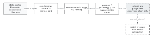
Thermal power counting chooses hard and soft regions; sum-integrals are split into vacuum and thermal parts, vacuum counterterms renormalize them, and mass, width, infrared, RG, and gauge checks bound the final observable. Solid connections show the primary relation; dashed outlines or arrows mark qualifications and failure boundaries. The diagram is schematic and not to scale.

The surrounding discussion supplies the relevant equations and checks in text form; the figure is a navigational summary.

Exercise

Show dimensionally that $T\int\mathrm d^3k\log(1+m_s^2/k^2)$ scales as $Tm_s^3$ after ultraviolet-overlap terms are subtracted.

Solution

Rescale $\mathbf k=m_s\mathbf q$. The measure supplies $m_s^3$, the logarithm becomes dimensionless, and the prefactor supplies $T$. Polynomial ultraviolet pieces correspond to hard-region overlap and are removed by the displayed subtraction and matching; the remaining soft contribution is proportional to $Tm_s^3$.

References

• Ginsparg, Paul. “First- and Second-Order Phase Transitions in Gauge Theories at Finite Temperature.” Nuclear Physics B 170 (1980): 388–408. doi:10.1016/0550-3213(80)90418-6.
• Linde, A. D. “Infrared Problem in Thermodynamics of the Yang–Mills Gas.” Physics Letters B 96, nos. 3–4 (1980): 289–292. doi:10.1016/0370-2693(80)90769-8.