Scale Hierarchies in Hot Gauge Theories

The central skill in hot gauge theory is to identify which degrees of freedom remain dynamical at the scale probed by an observable. In an asymptotically hot plasma, the hierarchy $T$, $gT$, and $g^2T$ separates hard particles, electrically screened collective fields, and a confining three-dimensional magnetic sector. The hierarchy organizes calculations; it does not assert that QCD at every experimentally accessible temperature is numerically weakly coupled.

Required background. QCD fields, scales, and the perturbative domain supplies the gauge and matter content, while scale and power counting supplies thermal loop counting. Helpful background. Modes, matching, and power counting develops the general EFT construction used here.

Hard, electric, and magnetic scales

Consider an equilibrium $\mathrm{SU}(N_c)$ gauge theory with $N_f$ light fermions and $g(T)\ll1$. Typical thermal particles have momentum $p\sim T$, occupation $f(p)\sim1$, and number density $n\sim T^3$. A soft gauge field with $K^\mu=(\omega,\mathbf{k})\sim gT$ polarizes this hard population. Its one-loop self-energy is enhanced to

$$\Pi_{\mathrm{HTL}}\sim g^2\int\frac{d^3p}{p}\,f(p)\sim g^2T^2,$$

so $K^2$ and $\Pi_{\mathrm{HTL}}$ are the same order. Bare perturbation theory must therefore be reorganized. For QCD at zero chemical potential,

$$m_D^2=g^2T^2\left(\frac{N_c}{3}+\frac{N_f}{6}\right)+O(g^3T^2)$$

defines the leading Debye scale. The static temporal field $A_0$ is electrically screened at distances $r\sim(gT)^{-1}$.

Static transverse magnetic fields have no perturbative mass term. After harder modes are removed, their three-dimensional coupling is $g_M^2\sim g^2T$, which itself has dimensions of mass. At momenta $k\sim g^2T$, the dimensionless interaction strength $g_M^2/k$ is order unity: the magnetostatic sector is intrinsically nonperturbative. This is the origin of the Linde obstruction rather than a defect of a particular gauge choice.

Fermions have no zero Matsubara mode and hence no static $gT$ or $g^2T$ field in the dimensionally reduced theory. They still matter through matching coefficients and as hard quasiparticles in real-time kinetic theory.

Frequencies, mean free paths, and formation times

Momentum alone does not select an effective description. A soft real-time disturbance with $\omega,k\sim gT$ belongs to HTL theory, whereas a static correlator at the same spatial momentum belongs to EQCD. Collisions of hard quasiparticles introduce parametrically longer times. Up to logarithms,

$$\gamma_{\mathrm{hard}}\sim g^2T\ln(1/g),\qquad t_{\mathrm{large\ angle}}\sim\frac{1}{g^4T\ln(1/g)}.$$

The first scale describes frequent soft color-randomizing kicks; the second reflects the accumulation needed for order-one momentum deflection. Transport coefficients are large because conserved quantities relax on the latter time scale. For example, dimensional analysis and kinetic power counting give

$$\eta\sim\frac{T^3}{g^4\ln(1/g)}$$

at leading logarithmic order.

Nearly collinear radiation supplies a further scale. A daughter with transverse momentum $k_\perp$ and longitudinal energy $p$ has an energy mismatch $\delta E\sim k_\perp^2/[2p\,x(1-x)]$, so its formation time is $t_{\mathrm{form}}\sim1/\delta E$. Multiple soft scatterings occur during formation and interfere—the Landau–Pomeranchuk–Migdal effect. A leading-order kinetic theory must resum this interference rather than add independent Bethe–Heitler emissions.

For anisotropic distributions, the state brings another dimensionless datum. Directional gradients of $f(\mathbf p)$ can make a transverse eigenvalue of the hard-loop inverse propagator negative, generating a growth rate $\gamma_{\mathrm{inst}}\sim gT$ for sufficiently strong anisotropy. This is not an equilibrium scale and requires the generalized hard-loop description on the instabilities page.

Hot-gauge plasma validity table

The table is a compact specification of what must accompany a hot-gauge claim. “Physical” means that the final quantity can be defined gauge invariantly; gauge-fixed intermediate propagators remain legitimate when their dependence cancels or the pole is protected at the stated order.

Observable or question	Dominant scale and time	Effective description and nominal order	Required matching input	Gauge status	Nonperturbative input or numerical test	Leading unresolved uncertainty
Pressure through $g^5T^4$	$T$ and $gT$, static	Four-dimensional QCD matched to EQCD	Running $g$, masses, factorization scale, EQCD coefficients	Physical after scale cancellation	Perturbative coefficient checks and renormalization-scale variation	Convergence at moderate coupling
Pressure at $g^6T^4$	$g^2T$, static	MQCD contribution plus hard/electric matching	EQCD-to-MQCD matching and subtraction convention	Physical	Three-dimensional lattice vacuum energy	Nonperturbative constant and higher orders
Debye screening	$k\sim gT$, static	EQCD or static HTL at leading order	$m_E^2$, operator definition	Physical only for a specified gauge-invariant screening channel; $\Pi_{00}(0,0)$ is an LO diagnostic	Continuum EQCD/lattice screening spectrum	Higher-order and operator dependence
Plasmon dispersion and Landau cut	$\omega,k\sim gT$	Retarded HTL	Hard distribution and retarded prescription	Poles are controlled order by order; spectral components can be gauge-fixed intermediates	Ward identities, sum rules, pole/cut numerical reconstruction	Collision broadening beyond collisionless HTL
Ultrasoft topology change	$k\sim g^2T$, $\omega\ll k$	Bödeker Langevin theory at leading log	Color conductivity matched through kinetic theory	Gauge-invariant diffusion rate	Regulated real-time classical lattice plus continuum matching	Beyond-leading-log conductivity and lattice extrapolation
Shear viscosity or charge diffusion	$p\sim T$, $t\sim[g^4T\ln(1/g)]^{-1}$	Linearized effective kinetic theory	Screened $2\leftrightarrow2$, LPM $1\leftrightarrow2$, conserved zero modes	Physical	Variational convergence, cutoff cancellation, collision-operator conservation	Higher orders and extrapolation to realistic coupling
Momentum broadening $\hat q$	hard trajectory, transverse kicks from $gT$ to $T$	Wilson-line definition; perturbative/EQCD factorization by regime	Representation, trajectory, rapidity and renormalization conventions	Physical only after operator and scheme are fixed	Lattice EQCD where applicable; cutoff and sum-rule checks	Matching across soft/hard scales and phenomenological model dependence
Anisotropic instability	$k,\gamma\sim gT$ initially	Anisotropic hard loops; classical-statistical nonlinear evolution	Full $f(\mathbf p)$, seed spectrum, expansion and backreaction	Growth of gauge-invariant field energy is physical; mode amplitudes are gauge dependent	Lattice-spacing/volume/velocity-grid convergence and energy conservation	Quantum corrections, saturation, expansion, and relation to thermalization

The entries follow the scale analysis of Braaten and Pisarski 1990, pp. 569–634, the static factorization of Braaten and Nieto 1996, §§ II–IV, and the kinetic construction of Arnold, Moore, and Yaffe 2003, §§ 1–2. Each later page links back here because changing the observable or its kinematics can change the correct row.

A routing example

Suppose one is asked for “the screening length.” That wording is incomplete. The leading static color-electric diagnostic $m_D^{-1}\sim(gT)^{-1}$ follows from HTL/EQCD, but an asymptotically long spatial correlator can be dominated by the lightest gauge-invariant three-dimensional state and can therefore probe $g^2T$. A real-time magnetic disturbance instead experiences Landau damping and collisions. The correct calculation begins by specifying operator, frequency, momentum, and asymptotic distance—not by choosing a familiar mass formula.

Where the hierarchy can fail

The expansion requires $g\ll1$ and well-separated scales. Large logarithms may need resummation; anisotropy and high occupancy may invalidate equilibrium HTL; masses or chemical potentials add scales; and observables can receive comparable contributions from more than one region. Renormalization-scale variation is informative but does not prove convergence. Agreement with data at one temperature also does not validate the parametric hierarchy.

The most defensible statement at phenomenological coupling is therefore conditional: within a specified truncation and matching prescription, the result gives a weak-coupling benchmark. It is not automatically a first-principles determination of the QCD matter created in a collision.

The equilibrium weak-coupling hierarchy is easiest to read from left to right, while keeping the anisotropic-state branch separate.

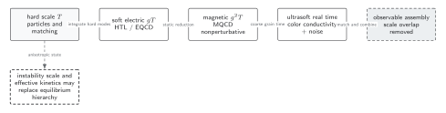
The solid sequence displays the parametric equilibrium hierarchy $T\gg gT\gg g^2T$ and the longer time scale controlled by color conductivity and noise. HTL and EQCD share the soft electric scale but answer real-time and static questions, respectively. The dashed branch warns that a sufficiently anisotropic state need not follow the equilibrium sequence. The diagram is schematic and not to scale; useful separation requires $g\ll1$.

In text, match hard modes into an observable-appropriate soft theory, treat the magnetic $g^2T$ sector nonperturbatively when it contributes, and cancel factorization-scale dependence when assembling the result. The hierarchy alone does not select HTL, EQCD, kinetic theory, or Bödeker dynamics without the observable and state.

Exercises

1. Locate the magnetic breakdown. In three-dimensional Yang–Mills theory, show that an $L$-loop correction at momentum $k$ is organized by powers of $g_M^2/k$. What happens at $k\sim g^2T$?

Solution

In three dimensions $[g_M^2]=1$. With $k$ the only infrared scale, every added interaction loop contributes a dimensionless factor proportional to $g_M^2/k$. Since matching gives $g_M^2\sim g^2T$, all loop orders become comparable at $k\sim g^2T$. No finite perturbative truncation controls that sector.

2. Estimate viscosity. Take a hard number density $n\sim T^3$, momentum per particle $p\sim T$, and transport mean free time $t_{\rm tr}\sim[g^4T\ln(1/g)]^{-1}$. Recover the parametric shear viscosity.

Solution

Kinetic theory gives $\eta\sim n\,p\,t_{\rm tr}$. Substitution yields $\eta\sim T^3 T/[g^4T\ln(1/g)]=T^3/[g^4\ln(1/g)]$, up to a dimensionless coefficient obtained by solving the linearized collision equation.

Continue to EQCD and MQCD for static matching or to HTL theory for soft real-time response.

References

• Arnold, Peter, Guy D. Moore, and Laurence G. Yaffe. “Effective Kinetic Theory for High Temperature Gauge Theories.” Journal of High Energy Physics 2003, no. 1 (2003): 030. DOI.
• Arnold, Peter, Guy D. Moore, and Laurence G. Yaffe. “Transport Coefficients in High Temperature Gauge Theories: (I) Leading-Log Results.” Journal of High Energy Physics 2000, no. 11 (2000): 001. DOI.
• Braaten, Eric, and Agustín Nieto. “Free Energy of QCD at High Temperature.” Physical Review D 53, no. 6 (1996): 3421–3437. DOI.
• Braaten, Eric, and Robert D. Pisarski. “Soft Amplitudes in Hot Gauge Theories: A General Analysis.” Nuclear Physics B 337, no. 3 (1990): 569–634. DOI.
• Linde, Andrei D. “Infrared Problem in Thermodynamics of the Yang–Mills Gas.” Physics Letters B 96, no. 3–4 (1980): 289–292. DOI.