

Keldysh Vertices and Causal Diagrammatics
In the basis, unitarity becomes a vertex selection rule: every closed-system interaction vertex contains at least one leg. The causal diagram rules are derived systematically in Kamenev and Levchenko 2009, §§ 2.2–2.4. Retarded and advanced lines then impose time inequalities that make many apparent branch diagrams vanish before any momentum integral is evaluated.
Required background. Use the retarded/advanced/Keldysh rotation, largest-time identities, and momentum-space Feynman rules.
Quartic vertices in the declared normalization
Section titled “Quartic vertices in the declared normalization”For
substitute . The elementary identity
gives
There are and vertices and no or vertex. Their numerical factors depend on whether identical-leg factorials are included in the vertex rule, so the safest check is to differentiate the displayed action with respect to the labeled fields. A rotation would redistribute powers of two.
More generally,
containing only odd powers of for a local potential. This proves term by term. Derivative interactions require integration by parts and contact terms but obey the same normalization condition.
Propagator index flow
Section titled “Propagator index flow”The free bosonic matrix is
There is no line. An line is retarded in the first time relative to the second; an line is advanced. Following a closed chain of retarded lines gives
which is impossible for distinct times. Therefore a closed retarded loop vanishes. This causal proof is independent of equilibrium distributions and often removes diagrams that would otherwise cancel only after a branch sum.
At coincident times the strict inequalities become ambiguous. A consistent contour regulator, canonical contact terms, and the chosen value of determine possible local remnants. Declaring every retarded loop zero without checking equal-time terms can discard anomaly, Jacobian, or derivative-vertex contributions.
The diagram provides the upstream checks for every causal diagram. The difference action fixes the vertices, the propagator matrix fixes index flow, and equal-source normalization forbids structures that would violate the largest-time identity.
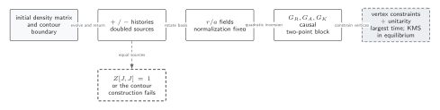
For a local closed-system interaction written as , the declared rotation fixes the allowed vertex index structures and their normalization; kernel inversion fixes only the two-point propagator block. Propagator support plus the largest-time identity then removes acausal diagrams. KMS further relates thermal correlators and vertices only in equilibrium; it is not a generic nonequilibrium selection rule. The diagram is schematic and not to scale.
The sections Quartic vertices in the declared normalization, Propagator index flow, and Causal construction rules supply the text and equation equivalent, including the diagrammatic rules, of the central and final boxes.
Checked one-loop examples
Section titled “Checked one-loop examples”Retarded cycle. Consider two vertices connected so that both internal lines point retardedly around the loop. The integrand contains , which is zero away from . With a prescription appropriate to a strictly ordered contour and no derivative contact term, the loop vanishes exactly.
Statistical tadpole. The vertex can contract two legs into the line, leaving one and one external leg. This generates a local retarded self-energy proportional to the statistical equal-time correlator. It does not vanish: the loop is statistical, not a closed retarded cycle. This distinction prevents the overstatement that “all loops vanish” in the basis.
Causal construction rules
Section titled “Causal construction rules”- Write the branch action and perform the declared rotation algebraically.
- Label each vertex by its number and position of legs.
- Reject any contraction requiring an propagator.
- Orient every propagator by its causal support.
- Search for incompatible closed time inequalities.
- Treat coincident-time and derivative contact terms separately.
- Only then evaluate momenta and statistical factors.
Largest-time cancellation survives out of equilibrium. KMS identities and thermal cutting simplifications do not; inserting a Bose distribution in a causal proof is unnecessary and can hide an unjustified equilibrium assumption.
Failure tests
Section titled “Failure tests”- Reconstruct the vertex by summing all assignments and compare with the result.
- Set and demand that the complete action, including counterterms, vanishes.
- Verify every retained response diagram has a directed path from each physical source insertion to the measured operator.
- Change the equal-time prescription and confirm that only identified contact terms change.
- Check that self-energy components obey the same Hermiticity and causal identities as the propagators.
Exercise
Section titled “Exercise”Why can a diagram containing a line evade the closed-retarded-loop argument?
Solution
is statistical and has no one-way step-function support. Replacing one link in a cycle by removes one strict time inequality, so the remaining retarded inequalities can be consistent. The diagram may still vanish by symmetry or vertex parity, but not by the closed-retarded-cycle proof alone.
Continue
Section titled “Continue”Use these vertices with contour-source derivatives on nonlinear response. Impose KMS relations only after equilibrium has been established.
References
Section titled “References”- Chou, K.-C., Su, Z.-B., Hao, B.-L., and Yu, L. (1985). “Equilibrium and Nonequilibrium Formalisms Made Unified.” Physics Reports 118, 1–131. DOI.
- Kamenev, A., and Levchenko, A. (2009). “Keldysh Technique and Non-Linear Sigma-Model: Basic Principles and Applications.” Advances in Physics 58, 197–319. arXiv:0901.3586; DOI.