Euclidean Fields and Classical Statistical Systems

A positive regulated Euclidean functional weight has the mathematics of a classical statistical field ensemble in the same number of Euclidean dimensions. This correspondence transfers partition functions, static correlations, critical behavior, and transfer-matrix data. It does not by itself supply a Lorentzian state, a causal correlator, or real-time dynamics; those require reflection positivity and reconstruction or a separately defined continuation.

The additional hypotheses required to reconstruct a relativistic quantum theory from Euclidean functions are stated by Osterwalder and Schrader 1973, pp. 83–112.

Required background. Wick Rotation and Analytic Continuation states the analytic data required to relate signatures. Statistical Ensembles and Field Configurations defines the ensemble measure. Helpful background. Reflection Positivity within Osterwalder–Schrader Reconstruction explains the positivity condition needed for a unitary Lorentzian interpretation.

The regulated correspondence

Consider a real scalar on a $D$-dimensional Euclidean lattice,

$$S_E[\phi]=a^D\sum_x \left[ \frac12\sum_{i=1}^{D}(\nabla_i\phi_x)^2 +\frac{r}{2}\phi_x^2+\frac{u}{4!}\phi_x^4 \right].$$

If $u>0$ and the integration cycle is real, the normalized functional measure

$$\mathrm dP[\phi] =\frac1Z\prod_x\mathrm d\phi_x\,e^{-S_E[\phi]}$$

is a classical probability measure. The same formula can be read as the continuum limit of a soft-spin statistical model with dimensionless Hamiltonian $\mathcal H/T=S_E$. Thus source derivatives, connected correlations, correlation lengths, and static universality classes are shared objects.

This statement is exact at the chosen regulator. The continuum notation

$$Z=\int\mathcal D\phi\,e^{-\int\mathrm d^D x\, [\frac12(\partial\phi)^2+\frac r2\phi^2+\frac{u}{4!}\phi^4]}$$

is shorthand until its measure and ultraviolet prescription are fixed. Couplings also carry different engineering units in a classical lattice Hamiltonian and a continuum Euclidean action; the dimensionless exponent, not a bare symbol such as $u$, is what is directly identified.

Transfer matrices and the extra interpretation

Choose one Euclidean direction as $\tau$. When the action is local in that direction and reflection positive, a transfer operator $\mathsf T$ can be constructed with

$$\mathsf T=e^{-aH},$$

where $H$ is a positive quantum Hamiltonian after normalization. Correlations separated by $n$ slices have the spectral form

$$\langle\mathcal O(n a)\mathcal O(0)\rangle_E =\frac1Z\operatorname{Tr} \left(\mathsf T^{N-n}\mathcal O\mathsf T^n\mathcal O\right).$$

This yields exponential decay governed by transfer-matrix gaps. It is stronger than merely observing a positive Boltzmann weight: reflection positivity, locality, boundary conditions, and a controlled continuum limit are part of the reconstruction. A sign-problem weight or a contour-deformed integral can compute legitimate observables without defining a positive classical ensemble on its displayed variables.

What static correspondence preserves

The dictionary preserves the following finite-regulator quantities when their normalizations are matched:

Euclidean field language	Classical statistical language	Check
$Z[J]$	source-dependent configurational partition function	$Z[0]$ normalizes the measure
connected Euclidean correlator	connected equilibrium correlation	source derivatives of $\log Z$ agree
inverse spatial correlation length	screening gap	exponential and second-moment estimators converge together
relevant Euclidean coupling	tuning parameter near a critical surface	dimensionless scaling variable agrees
Euclidean finite-size scaling	finite-size scaling of the statistical model	universal exponents agree after metric factors

The correspondence is especially powerful near a continuous transition, where long-distance static observables forget many microscopic details. But it does not make ultraviolet normalizations universal, nor does it identify the quantum time evolution of the $D$-dimensional statistical model.

What the correspondence loses

An unordered Euclidean correlator does not specify a retarded function. Causal support, commutator signs, the $i0$ prescription, and the state enter the Lorentzian boundary value. Even when exact Euclidean data determine an analytic function uniquely under appropriate growth hypotheses, a finite noisy data vector leads to an ill-posed inverse problem.

Nor does static universality determine dynamic universality. The same equilibrium free energy may be paired with relaxational, conserved, reversible, or Hamiltonian dynamics, producing different dynamic exponent $z$. Those choices are developed in Critical and Stochastic Dynamics.

For a compact Euclidean time circle of circumference $\beta$, the field boundary condition records statistics and trace insertions. It cannot be chosen from the classical analogy alone; Thermal Boundary Conditions and Graded Traces distinguishes thermal and graded cases.

Failure tests

Positivity test. If the weight is complex or changes sign, do not call it a classical probability distribution. Reweighting identities may remain algebraically true, but their variance and overlap must be assessed separately.

Reflection test. A positive pointwise weight need not be reflection positive. Test the quadratic form $\langle(\Theta F)F\rangle_E\ge0$ for observables supported on one side of a reflection before claiming a positive Hilbert-space reconstruction.

Dynamics test. Replace a proposed real-time conclusion by two distinct stochastic dynamics with the same stationary measure. If they give different time dependence, the equilibrium Euclidean measure did not determine that conclusion.

The schematic below organizes the relationships used on this page. Inspect it with this question in mind: How do Euclidean configurations, correlations, Gaussian fluctuations, phases, and thermodynamic limits relate?

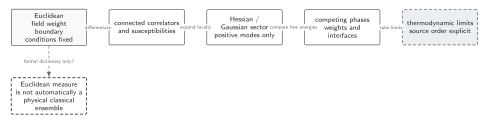
A Euclidean weight defines correlations; a positive Hessian licenses Gaussian fluctuations locally, while phase coexistence and spontaneous breaking require a separately ordered thermodynamic and source limit. Solid connections show the primary relation; dashed outlines or arrows mark qualifications and failure boundaries. The diagram is schematic and not to scale.

The surrounding discussion supplies the relevant equations and checks in text form; the figure is a navigational summary.

Exercise

For the Gaussian action $S_E=\frac12\int\mathrm d^D x[(\nabla\phi)^2+m^2\phi^2]$, show that the spatial correlation length is $m^{-1}$ while no real-time damping rate is fixed.

Solution

The momentum-space covariance is $(\mathbf k^2+m^2)^{-1}$, whose nearest complex spatial-momentum singularities are at $\lvert\operatorname{Im}\mathbf k\rvert=m$; the position-space correlator therefore decays as $e^{-mr}$ times a power. One may impose Hamiltonian evolution, overdamped Langevin evolution, or another dynamics with this same equilibrium covariance, and they have different frequency dependence. Hence $m^{-1}$ is a static screening length, not a damping time.

References

• Glimm, James, and Arthur Jaffe. Quantum Physics: A Functional Integral Point of View. 2nd ed. New York: Springer, 1987. doi:10.1007/978-1-4612-4728-9.
• Osterwalder, Konrad, and Robert Schrader. “Axioms for Euclidean Green’s Functions.” Communications in Mathematical Physics 31 (1973): 83–112. doi:10.1007/BF01645738.
• Zinn-Justin, Jean. Quantum Field Theory and Critical Phenomena. 5th ed. Oxford: Oxford University Press, 2021. doi:10.1093/oso/9780198834625.001.0001.