

Initial Density Matrices and Contour Boundary Conditions
An initial density matrix is a boundary interaction at . Its quadratic part fixes the Gaussian mean and covariance; higher boundary vertices encode connected non-Gaussian cumulants. These data survive through retarded propagation and memory kernels, so a bulk action alone never specifies a nonequilibrium problem.
Required background. Use the closed-time-path generating functional for branch orientation and source signs.
Helpful background. Initial correlations in Kadanoff–Baym evolution shows how boundary cumulants enter later two-time equations.
Boundary action and density-matrix constraints
Section titled “Boundary action and density-matrix constraints”In the field basis, choose the field-independent normalization real and positive and write
is localized at . Hermiticity requires
or, in variables, . Trace normalization is instead the integrated condition
It does not imply . A diagonal density kernel is normally a nonconstant probability weight. By contrast, the bulk difference action vanishes pointwise on equal histories, and the complete contour integral obeys . The initial kernel and the normalized generating functional appear as distinct objects in Crossley, Glorioso, and Liu 2017, § II.A, pp. 32–35.
Where is nonzero, one may factor
This optional residual action has the pointwise-zero property because the essential diagonal probability has first been factored out. It should not be confused with the original .
Positivity is stronger still: for every wave functional , . Neither Hermiticity nor trace one proves it.
For one oscillator, a general centered Gaussian state is specified by
with
Write . For a real one-mode Gaussian covariance, and are the necessary and sufficient conditions for a positive density operator. Merely writing a positive Gaussian Wigner function does not replace the uncertainty condition. For a unit-mass oscillator, , and the statistical correlator carries all three entries:
For a field mode, replace by its canonical momentum and restore the kinetic normalization. The equal-time commutator fixes the corresponding spectral data independently.
Reconstructing the Gaussian kernel
Section titled “Reconstructing the Gaussian kernel”The reconstruction is most transparent through the Wigner function. With and
the inverse transform is an elementary Gaussian integral. It gives
The diagonal integral is one, and changing complex-conjugates the kernel. A second Gaussian integral gives , with equality exactly for a pure Gaussian state. Reading the same result as gives
The pure term is essential: it supplies the diagonal probability weight. In a field theory, a centered Gaussian has the same structure in kernel notation,
where the kernels are fixed by the field and momentum covariance matrices. Linear terms encode nonzero means. Hermiticity constrains their reality properties, while positivity imposes matrix inequalities that couple , , and ; they cannot be chosen independently.
Non-Gaussian boundary vertices
Section titled “Non-Gaussian boundary vertices”Connected initial -point functions require boundary vertices. A general expansion sums over every assignment,
Every time argument is . Pure- boundary vertices are allowed; the rule that every bulk dynamical vertex contains an field does not apply to the raw density kernel. A -symmetric state has no odd vertices but can have a connected four-point kernel. These boundary-localized kernels and their role in the interacting equilibrium limit are developed in Garny and Müller 2009, § II, pp. 2–4.
A useful positive example is a symmetric mixture of two translated Gaussian states,
If the centered kernel has , then
This state is normalized and positive by construction. Its position distribution has connected fourth cumulant , while begins with a quadratic correction followed by . Thus the first non-Gaussian boundary correction can be an all- vertex. Truncating that logarithm is a useful perturbative model, but the truncated expression must be rechecked for positivity and ultraviolet behavior.
The map below organizes the dependencies of a late-time response. Four solid arrows carry the declared state, boundary correlations, sources, and memory kernel into the observable; the dashed arrow marks the separate test required before claiming loss of memory.
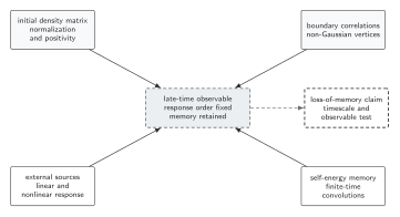
The solid arrows identify data on which the response calculation can depend, while the dashed outgoing arrow separates the calculated response from a later memory-loss claim. The initial density matrix fixes trace normalization, positivity, and boundary kernels, while non-Gaussian cumulants require additional contour vertices. Factorization or Gaussianity removes specific inputs only when imposed and checked; neither implies late-time loss of memory. The diagram is schematic and not to scale.
The sections Boundary action and density-matrix constraints, Reconstructing the Gaussian kernel, Non-Gaussian boundary vertices, and Preparation protocols and failure tests give the text and equation equivalent of the upper dependencies and their checks.
Thermal and squeezed-state checks
Section titled “Thermal and squeezed-state checks”For a thermal oscillator, , , , and . Substitution gives the normalized kernel
Its diagonal is visibly nonconstant. At zero temperature it reduces to the vacuum kernel .
For a pure squeezed oscillator state with squeeze parameter and angle chosen so ,
It saturates the uncertainty bound for every . Calling a thermal occupation would be wrong: field and momentum variances correspond to different effective energies. Free evolution rotates the squeezed ellipse and preserves its determinant, so unequal-time retains the phase information.
The thermal determinant is : equality holds in the zero-temperature vacuum, and the inequality is strict for . A thermal and a squeezed state can share one equal-time variance but not the full covariance.
Preparation protocols and failure tests
Section titled “Preparation protocols and failure tests”An imaginary-time segment prepares a thermal or Euclidean-correlated state. An adiabatic source prepares a different state and requires a scale separation. A sudden quench is a physical protocol, not a numerical convenience; it injects energy and high-frequency correlations. A finite switch-on must be included in the source history.
Test the state by:
- verifying the integrated diagonal trace, Hermiticity, and covariance positivity before evolution;
- checking that equal boundary fields leave the intended diagonal probability rather than forcing the boundary integrand to one;
- checking its ultraviolet tail against the renormalized vacuum behavior;
- moving while keeping the actual preparation protocol fixed;
- adding the first omitted connected cumulant; and
- evolving a purported interacting equilibrium state without a quench—any drift is an inconsistency or numerical error.
Exercises
Section titled “Exercises”Reconstruct and evolve a Gaussian state
Section titled “Reconstruct and evolve a Gaussian state”Starting from the Gaussian kernel above, verify trace normalization and Hermiticity. Then show that free evolution gives
where and . Can two states with the same but different have the same future ?
Solution
At , the kernel is the normalized Gaussian . Under exchange , changes sign; only the phase term changes sign, so the kernel is complex-conjugated. Free motion is . Symmetrizing the product gives the displayed expression. Different changes the coefficient of the sine–sine term, so equal alone cannot fix future statistical correlations.
Locate the first non-Gaussian vertex
Section titled “Locate the first non-Gaussian vertex”For the translated mixture above, expand through order and compute .
Solution
Using gives the all- quartic term in . Write the position random variable as , where is centered Gaussian with variance and with equal probability. Then and , so . The exact mixture is positive; a finite series for its logarithm is not automatically so.
Continue
Section titled “Continue”Use unitarity and largest-time identities to constrain the later dynamical sector without imposing a pointwise rule on the initial kernel, then follow boundary correlations into Kadanoff–Baym evolution.
References
Section titled “References”- Crossley, M., Glorioso, P., and Liu, H. (2017). “Effective Field Theory of Dissipative Fluids.” Journal of High Energy Physics 2017(09), 095. arXiv:1511.03646; DOI.
- Garny, M., and Müller, M. M. (2009). “Kadanoff–Baym Equations with Non-Gaussian Initial Conditions: The Equilibrium Limit.” Physical Review D 80, 085011. arXiv:0904.3600; DOI.
Further reading
Section titled “Further reading”- Chou, K.-C., Su, Z.-B., Hao, B.-L., and Yu, L. (1985). “Equilibrium and Nonequilibrium Formalisms Made Unified.” Physics Reports 118, 1–131. DOI.