Dynamical KMS and Topological Symmetries

Two symmetry structures coexist in thermal Schwinger–Keldysh hydrodynamics. A topological or BRST-like sector implements contour normalization and largest-time identities even away from equilibrium. Dynamical KMS is an additional discrete thermal transformation that combines imaginary thermal translation with an antiunitary operation. Conflating them incorrectly imposes equilibrium fluctuation–dissipation on generic driven states.

Required background. Schwinger–Keldysh Effective Actions for Fluids supplies the $r/a$ action. Unitarity, Normalization, and Largest-Time Identities derives the contour identities.

Helpful background. Detailed Balance and Fluctuation–Dissipation gives their classical stochastic counterpart.

What follows from unitarity

For identical sources on both contour legs,

$$Z[J,J]=1.$$

Consequently the effective action vanishes when every $a$ field and $a$ source vanishes. Correlators obey largest-time zeros, and the pure $a=0$ sector is topological in the sense that physical deformations common to both legs do not change the normalized functional.

In a nonlinear local path integral, nilpotent BRST-like charges can impose these identities off shell. Ghost fields represent the Jacobian of the stochastic or hydrodynamic change of variables. They decouple in some Gaussian additive-noise calculations, but that special simplification is not a license to omit them when the measure, constraints, or multiplicative noise is field dependent.

These statements use microscopic unitarity and the closed contour. They do not assume a Gibbs state.

The separation between contour normalization, largest-time identities, and additional thermal conditions is explicit in Crossley, Glorioso, and Liu 2017, §§2–3, Open PDF.

The classical dynamical-KMS map

Let $\Theta$ be the relevant antiunitary transformation, including time reversal and any necessary parity or charge conjugation. For a bosonic hydrodynamic field in a stationary thermal state, the classical-limit transformation has the schematic local form

$$\widetilde\phi_r(x)=\Theta\phi_r(x),$$ $$\widetilde\phi_a(x) = \Theta\phi_a(x) +i\,\Theta\mathcal L_\beta\phi_r(x),$$

where the transformed point includes $t\to-t$, $\beta^\mu=u^\mu/T$ is the thermal vector, and gauge-charged fields use a thermal gauge twist as well as $\mathcal L_\beta$. Signs depend on the intrinsic $\Theta$ parity and on the $a$ normalization; the invariant content is the imaginary translation by the thermal flow.

For global equilibrium $\beta^\mu$ is Killing. In local-equilibrium EFT it varies slowly, and invariance is imposed order by order in derivatives. Glorioso, Crossley, and Liu prove the equivalence of this classical dynamical symmetry to their local KMS condition and derive the entropy-current consequences Glorioso, Crossley, and Liu 2017, §§2–4 and 6, Open PDF.

Diffusion Ward identity

Apply the transformation to the quadratic diffusion EFT. Dynamical KMS pairs the dissipative term with the imaginary term, forcing the same $\sigma$ to appear in

$$\mathbf j_{\mathrm{diss}}=-\sigma\boldsymbol\nabla\mu$$

and

$$\left\langle\xi_i(x)\xi_j(x')\right\rangle =2T\sigma\delta_{ij}\delta(x-x').$$

Equivalently, its two-point Ward identity is the KMS fluctuation–dissipation relation. In the classical low-frequency limit,

$$G^S_{nn}(\omega,k) = -\frac{2T}{\omega}\operatorname{Im}G^R_{nn}(\omega,k),$$

because the site convention has $\rho=-2\operatorname{Im}G_R$. Substituting

$$G^R_{nn}=-\chi\frac{Dk^2}{-i\omega+Dk^2}$$

reproduces the positive symmetric correlator from the previous page.

At nonlinear order, the same symmetry relates response vertices and noise cumulants and yields generalized Onsager constraints. A local entropy current can be constructed order by order, but its representative is not unique and the symmetry does not prove global entropy monotonicity far from equilibrium.

BRST, KMS, and emergent supersymmetry

The normalization BRST charge and its KMS transform can combine into an $\mathcal N=2$-type topological supersymmetry in the classical statistical limit. The algebra closes on a thermal translation. This elegant structure depends on the classical limit, thermal assumptions, field content, and treatment of ghosts; it is not an exact supersymmetry of an arbitrary microscopic thermal QFT.

An anomaly can obstruct naive invariance or add inflow terms. A chemical potential requires the thermal twist. Spontaneous breaking can make the KMS symmetry act nonlinearly. At finite quantum frequency the imaginary translation is nonlocal when expanded in real time, so a finite local classical action captures only its derivative expansion.

The fluctuating-hydrodynamics and SK consistency reference keeps the normalization, KMS, positivity, and cutoff statements separate.

The upper-left label contains the distinction this page enforces: noise belongs to the fluctuating SK branch, but dynamical KMS is marked as an equilibrium condition. Inspect that qualifier before comparing this branch with extensions generated by genuinely new slow variables.

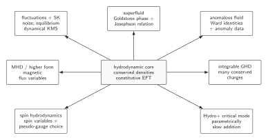
SK normalization and its topological implementation follow from unitarity of the closed time path. Dynamical KMS instead uses a thermal state, time reversal or its appropriate antiunitary generalization, and a local derivative expansion. The diagram is schematic and the branch labels logical ingredients, not an implication from noise to equilibrium.

In text: $S[\phi_r,0]=0$ and SK reality hold without thermal equilibrium; positivity constrains the imaginary part; dynamical KMS then relates dissipative and fluctuation coefficients when its thermal hypotheses apply. None of these statements creates a superfluid, anomaly, or other slow sector.

Exercise

For the diffusion correlator above, verify the classical KMS relation explicitly.

Solution

The imaginary part is

$$\operatorname{Im}G^R_{nn} = -\chi\frac{Dk^2\omega}{\omega^2+(Dk^2)^2}.$$

Therefore

$$-\frac{2T}{\omega}\operatorname{Im}G^R_{nn} = \frac{2T\chi Dk^2}{\omega^2+(Dk^2)^2} =G^S_{nn}.$$

The sign would fail if one combined the site retarded convention with a response convention taken from a source of opposite sign.

Common pitfalls

Deriving KMS from $Z[J,J]=1$. Normalization is state independent; KMS is thermal.

Dropping ghosts because they decouple quadratically. Nonlinear Jacobians and constraints can recouple them.

Using global-equilibrium KMS in a driven steady state. A driven state needs its own symmetry or fluctuation relation; a thermal one cannot be assumed.

Where this leads

Long-Time Tails and Fluctuation Renormalization uses KMS-matched nonlinear loops. Charged and Anomalous Hydrodynamics shows how thermal twists and anomalies qualify the symmetry.

References

• Crossley, Michael, Paolo Glorioso, and Hong Liu. 2017. “Effective Field Theory of Dissipative Fluids.” Journal of High Energy Physics 2017 (9): 095. DOI. Open PDF.

• Glorioso, Paolo, Michael Crossley, and Hong Liu. 2017. “Effective Field Theory of Dissipative Fluids (II): Classical Limit, Dynamical KMS Symmetry and Entropy Current.” Journal of High Energy Physics 2017 (9): 096. DOI. Open PDF.