

Fokker–Planck Evolution and Stationary Measures
The Fokker–Planck equation evolves the probability density induced by a stochastic differential equation. A formal zero mode of its operator is a physical stationary state only if it is nonnegative, normalizable, compatible with boundary currents, and selected uniquely—or with explicitly stated sector weights—by the dynamics.
Required background. Use Brownian motion, stochastic calculus, and Fokker–Planck equations and Langevin field equations.
Helpful background. Detailed balance and fluctuation–dissipation distinguishes equilibrium zero current from general stationarity.
Itô evolution and probability current
Section titled “Itô evolution and probability current”For the Itô process, following the drift–diffusion convention summarized in Risken 1989, ch. 3,
define . The probability density obeys
with
For fields, indices become spatial points and derivatives become functional derivatives. The formula depends on the stochastic convention when depends on ; converting a Stratonovich equation to Itô adds a noise-induced drift.
Normalization follows from . It therefore requires periodic, reflecting, decaying, or otherwise specified boundary conditions. Absorbing boundaries deliberately lose probability from the domain and describe first-passage rather than a normalized stationary ensemble.
Equilibrium gradient flow
Section titled “Equilibrium gradient flow”For additive mobility ,
with symmetric positive , the Gibbs density
has . This direct substitution is the equilibrium fluctuation–dissipation check. If depends on , the drift must include the convention-dependent derivative of needed to produce the intended current; writing alone is generally incomplete.
For a conserved field, the mobility is an operator such as . Its zero mode expresses exact conservation of the spatial integral of , so the stationary measure is conditioned on that conserved sector rather than unique over all field configurations.
The middle of the schematic distinguishes probability evolution from equilibrium. The Fokker–Planck operator follows from the declared stochastic prescription; a stationary measure is an outcome of its probability current, and detailed balance is the stronger zero-current condition.
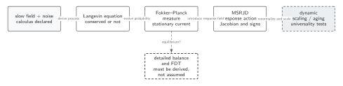
The Fokker–Planck equation and current depend on the Langevin drift, diffusion tensor, stochastic calculus, and boundary conditions. A stationary density may support a nonzero circulating current, so stationarity alone does not put the process on the detailed-balance branch. Normalizability, positivity, uniqueness, and ergodicity are additional questions. The diagram is schematic and not to scale.
The sections Itô evolution and probability current, Equilibrium gradient flow, and Stationarity, uniqueness, and ergodicity give the text and equation equivalent of the probability and equilibrium branches.
Checked Ornstein–Uhlenbeck process
Section titled “Checked Ornstein–Uhlenbeck process”For
the Fokker–Planck equation is
Setting gives
It is normalizable only for . For on the real line, the formal stationary solution is constant and nonnormalizable; diffusion has no equilibrium measure. On a finite periodic interval it is normalizable and unique, illustrating the role of domain and boundary conditions.
Stationarity, uniqueness, and ergodicity
Section titled “Stationarity, uniqueness, and ergodicity”permits nonzero circulating current in more than one dimension. Such a steady state is stationary but violates detailed balance and generally produces entropy. Uniqueness requires conditions such as confining drift, irreducible noise on the accessible state space, and no disconnected conserved sectors. Degenerate noise may leave invariant manifolds and multiple stationary measures.
A zero eigenvalue of the Fokker–Planck operator is not enough: check left/right eigenfunctions, normalization, spectral gap or mixing, and boundary domain. Near criticality the gap closes with system size, causing critical slowing down without necessarily destroying uniqueness at finite volume.
Use the stochastic and kinetic closure validity table to record convention, regulator, current, positivity, and convergence.
Failure tests
Section titled “Failure tests”- Derive the Fokker–Planck operator from the declared stochastic calculus.
- Substitute the proposed stationary density and evaluate the full current.
- Check normalization and boundary flux.
- Identify conserved sectors and degenerate-noise directions.
- Test uniqueness and mixing rather than assuming them from a long simulation.
- Vary the regulator for a field theory and retain induced counterterms.
Exercise
Section titled “Exercise”For the Ornstein–Uhlenbeck process, verify the stationary variance directly from the moment equation.
Solution
Itô’s lemma gives . Stationarity gives , agreeing with the Gaussian density.
Continue
Section titled “Continue”Represent the same process by the MSRJD response functional and decide whether its stationary state satisfies detailed balance.