Thermal Sum-Integrals and Vacuum Subtraction

A thermal sum-integral separates exactly into a zero-temperature contribution carrying the ordinary ultraviolet divergence and a state-dependent contribution weighted by Bose or Fermi distributions. The latter is ultraviolet finite for a massive or properly subtracted one-loop integrand because the occupations decay exponentially. Vacuum subtraction must preserve additive thermodynamic normalization and cannot be replaced by temperature-dependent counterterms.

The contour and distribution-function decompositions of thermal sum-integrals are derived in Laine and Vuorinen 2016, §§ 2.2–2.4.

Required background. Imaginary Time and Matsubara Frequencies fixes the sums. Dimensional Regularization and Minimal Subtraction fixes the regulator. Helpful background. Laurent Series, Poles, and Residues supplies the contour method.

Measures and master tadpole

In $d=4-2\epsilon$ spacetime dimensions define

$$\mathop{\sum\!\!\!\int}_P^B \equiv \bar\mu^{2\epsilon}T \sum_{n\in\mathbb Z} \int\frac{\mathrm d^{3-2\epsilon}p}{(2\pi)^{3-2\epsilon}}, \qquad P^2=\omega_n^2+\mathbf p^2,$$

with $\omega_n=2\pi nT$. The bar on $\mu$ indicates the chosen $\overline{\mathrm{MS}}$ convention; its precise $4\pi e^{-\gamma_E}$ factor must accompany quoted coefficients.

The bosonic tadpole is

$$I_B(m)=\mathop{\sum\!\!\!\int}_P^B\frac1{P^2+m^2}.$$

Performing the Matsubara sum gives

$$I_B(m)= \bar\mu^{2\epsilon} \int\frac{\mathrm d^{3-2\epsilon}p}{(2\pi)^{3-2\epsilon}} \left[ \frac1{2E_{\mathbf p}} +\frac{n_B(E_{\mathbf p})}{E_{\mathbf p}} \right].$$

The first term is the vacuum tadpole and contains the ultraviolet pole. The second is the finite thermal part. For $m=0$ in dimensional regularization the scaleless vacuum piece vanishes and

$$I_B(0)=\int\frac{\mathrm d^3p}{(2\pi)^3} \frac{n_B(p)}p=\frac{T^2}{12}.$$

“Scaleless equals zero” is a regulator statement combining ultraviolet and infrared analytic continuation; it is not proof that the vacuum fluctuation never existed.

Contour and spectral derivations

For an eligible function $f$,

$$T\sum_n f(i\omega_n) =\frac1{2\pi i}\oint_{\mathcal C_B} \mathrm dz\,n_B(z)f(z).$$

Deforming $\mathcal C_B$ to the singularities of $f$ produces the vacuum residues plus thermal weights. An equivalent spectral identity is

$$\mathop{\sum\!\!\!\int}_P^B G_E(P) =\int_{\mathbf p}\int\frac{\mathrm d\omega}{2\pi} \left[\frac12+n_B(\omega)\right] \rho(\omega,\mathbf p)$$

with parity and convergence understood. The contour arc, branch cuts, and subtractions must be checked; otherwise the “thermal part” can lose a polynomial contact term.

Trace log and free energy

For one real scalar,

$$\mathcal F_0(T,m)= \frac12\mathop{\sum\!\!\!\int}_P^B\log(P^2+m^2).$$

Differentiating yields $\partial\mathcal F_0/\partial m^2=I_B/2$. Integrating back gives

$$\mathcal F_0= \frac12\int_{\mathbf p}E_{\mathbf p} +T\int_{\mathbf p}\log(1-e^{-\beta E_{\mathbf p}}) +C,$$

where $C$ is fixed by the vacuum and pressure normalization. Dropping the first term is a chosen vacuum subtraction; dropping an arbitrary $T$-dependent constant would change entropy and energy.

Thermal perturbation and renormalization table

Use this table to keep state-independent ultraviolet renormalization separate from thermal populations and from reorganizations that add and subtract the same medium-dependent term.

Contribution	Typical origin	UV treatment	Thermal interpretation	Common double count
vacuum integral	$\tfrac12$, zero-point, or $T\to0$ part	ordinary local counterterms	state independent	subtracting it again after matching
thermal occupation	$n_B$ or $n_F$	finite after matched subtractions	state-dependent population	calling it a new UV counterterm
bosonic zero mode	$n=0$ term	same UV theory; separate IR reorganization	static infrared sector	including both bare and screened propagators
resummation insertion	added thermal mass or self-energy	add and subtract consistently	reorganizes soft counting	omitting the subtraction vertex
running parameter	vacuum RG and matched EFT coefficients	declared scheme and scale	cancels explicit scale dependence	varying scale in only one piece
imaginary part/cut	retarded boundary value	renormalize real and imaginary structure consistently	width or inclusive rate after KMS weights	counting a cut and kinetic process twice

This is the canonical semantic table for the chapter. Later pages link here when distinguishing UV subtraction, thermal reorganization, and physical interpretation.

Checks

• Take $T\to0$ and recover the regulated vacuum integral.
• Differentiate a trace log and recover the tadpole.
• Evaluate the thermal tadpole by both contour and occupation methods.
• Isolate the bosonic $n=0$ term before any small-mass expansion.
• Carry additive constants consistently into pressure and thermodynamic derivatives.

The schematic below organizes the relationships used on this page. Inspect it with this question in mind: How does a thermal loop calculation pass from scale counting to a physical observable?

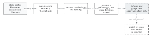
Thermal power counting chooses hard and soft regions; sum-integrals are split into vacuum and thermal parts, vacuum counterterms renormalize them, and mass, width, infrared, RG, and gauge checks bound the final observable. Solid connections show the primary relation; dashed outlines or arrows mark qualifications and failure boundaries. The diagram is schematic and not to scale.

The surrounding discussion supplies the relevant equations and checks in text form; the figure is a navigational summary.

References

• Kapusta, Joseph I., and Charles Gale. Finite-Temperature Field Theory: Principles and Applications. 2nd ed. Cambridge: Cambridge University Press, 2006. doi:10.1017/CBO9780511535130.
• Laine, Mikko, and Aleksi Vuorinen. Basics of Thermal Field Theory. Cham: Springer, 2016. doi:10.1007/978-3-319-31933-9; Open PDF.