

Imaginary Time and Matsubara Frequencies
When equilibrium correlators admit the required Euclidean continuation and field representation, the KMS boundary relation becomes a compact Euclidean-time circle of circumference . In the ordinary thermal trace, bosonic fields are periodic and fermionic fields are antiperiodic, so their Fourier modes have frequencies and , respectively. This discrete spectrum replaces the vacuum energy integral; the ordinary bosonic zero mode is often the source of thermal infrared enhancement.
The imaginary-time construction and its connection to real-time thermal functions are derived in Landsman and van Weert 1987, §§ 2.2–2.4, pp. 157–183.
Required background. Thermal Density Operators and the KMS Condition supplies the imaginary shift. Wick Rotation and Analytic Continuation supplies the Euclidean continuation. Helpful background. Laurent Series, Poles, and Residues supports contour evaluation of thermal sums.
The thermal circle and its Fourier modes
Section titled “The thermal circle and its Fourier modes”Algebraic KMS by itself does not manufacture a Euclidean path integral or a field-mode expansion. The formulas below assume an eligible Euclidean correlator or field representation, a declared operator parity and trace insertion, and the displayed compact-time Fourier convention.
For , expand a periodic bosonic field as
An antiperiodic fermion has
The prefactor is the inverse-transform normalization used here; a source may distribute factors of differently. Orthogonality reads
The global Lorentzian Fourier convention is inherited, but the Euclidean thermal transform is declared independently because is compact and the sign of varies across the literature.
Free thermal propagators
Section titled “Free thermal propagators”For a real scalar with Euclidean action
the Matsubara propagator is
Transforming back gives, for ,
At equal time,
which separates vacuum and thermal occupation. Periodicity follows because .
For a free Dirac field,
the inverse operator is in the displayed transform convention. With , its Gaussian propagator is
Euclidean gamma-matrix and Green-function sign conventions must be translated together before comparing numerators. The occupation factor can be checked without spinor algebra. For one fermionic mode , define
Then
Because , this obeys . The limits and both recover the Fermi occupation and give the canonical discontinuity .
Thermal sums from contour residues
Section titled “Thermal sums from contour residues”A bosonic Matsubara sum can be written schematically as
where encloses the poles of at . Deforming the contour expresses the result as residues or discontinuities of , plus any contribution at infinity. The contour orientation, singularities, and falloff are part of the derivation. Replacing by without changing the energy argument and boundary conditions is only a mnemonic.
Zero modes and chemical shifts
Section titled “Zero modes and chemical shifts”In the ordinary thermal spin structures used above, only bosons have an mode. For momenta , that bosonic mode behaves as a -dimensional classical field and can invalidate naive loop counting. Bosonic Zero Modes and Infrared Breakdown diagnoses the failure, while Modes, Matching, and Power Counting constructs the dimensionally reduced description. Periodic fermions in a supertrace instead have integer modes and can possess fermion zero modes; Thermal Boundary Conditions and Graded Traces explains why that sector is not an ordinary thermal ensemble. Thermal Propagators and Spectral Representations continues from these discrete Euclidean modes to the shared thermal spectral function.
A chemical potential can be represented either by evolving with or by a shift of the Euclidean derivative. For a field of charge , a common convention gives
so the displayed modes obey . Equivalently, after removing the connection the complex frequencies are for a boson. The sign depends on the charge, transform, and covariant-derivative conventions and must be derived from the displayed grand-canonical action, not memorized.
Checks and pitfalls
Section titled “Checks and pitfalls”- Verify periodicity or antiperiodicity after transforming back to .
- Recover the zero-temperature energy integral as .
- Check equal-time occupation factors against canonical quantization.
- Isolate the bosonic zero mode before infrared expansion.
- State whether a chemical potential appears as a twist or a frequency shift.
- Do not continue a finite noisy Matsubara data set as though it were an exact analytic function.
The lower panel makes the causal order explicit: a Euclidean representation, parity, and trace insertion fix the circle monodromy, and the monodromy fixes the Matsubara lattice and zero-mode sector.
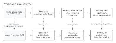
The positive-strip KMS boundary relation is common equilibrium input, but the mode expansion requires the additional Euclidean gate shown in the lower panel. For the ordinary heat trace, bosonic periodicity gives integer modes and permits a zero mode, while fermionic antiperiodicity gives half-integer modes. Conserved or graded insertions alter the monodromy and hence the lattice; algebraic KMS alone does not select a field path integral. The diagram is schematic and not to scale.
The surrounding formulas develop the transform normalization, propagators, and residue checks that follow downstream from the mode sectors summarized in the figure.
Exercise
Section titled “Exercise”For fermionic , evaluate
by contour residues. State the summation kernel, contour orientation, physical poles, and zero-temperature limit.
Solution
Use
The poles of at have residue , so a counterclockwise contour around them gives
Assuming the large arcs vanish, deforming the contour outward reverses the small contours around the physical poles of at . Their residues are and , respectively. Since ,
As , and the result approaches , the zero-temperature energy integral. The minus residue of the fermionic kernel is the sign that distinguishes this answer from the bosonic sum.
References
Section titled “References”- Landsman, N. P., and Ch. G. van Weert. “Real- and Imaginary-Time Field Theory at Finite Temperature and Density.” Physics Reports 145, nos. 3–4 (1987): 141–249. doi:10.1016/0370-1573(87)90121-9.
Further reading
Section titled “Further reading”- Kapusta, Joseph I., and Charles Gale. Finite-Temperature Field Theory: Principles and Applications. 2nd ed. Cambridge: Cambridge University Press, 2006. doi:10.1017/CBO9780511535130.
- Le Bellac, Michel. Thermal Field Theory. Cambridge: Cambridge University Press, 1996. doi:10.1017/CBO9780511721700.