Quenches, Coarsening, and Aging

After a quench into an ordered phase, domains grow and defects annihilate while the system remains out of equilibrium. The characteristic length may obey dynamic scaling, but two-time observables depend separately on observation time and waiting time. This aging behavior violates time-translation invariance and cannot be fitted by equilibrium fluctuation–dissipation without an explicit nonequilibrium qualification.

Required background. Use dynamic scaling and critical slowing down and the Landau–Ginzburg functional.

Helpful background. Nonthermal fixed points and wave turbulence treats scaling regimes whose degrees of freedom and conservation constraints differ from classical domain coarsening.

Domain-growth scaling

For a scalar order parameter quenched below its critical temperature, the single-length scaling hypothesis reviewed in Bray 1994, §§ II–III is

$$S(k,t)=L(t)^d f_S(kL(t)),$$

where $S$ is the equal-time structure factor. This implies collapse only after microscopic interface width and initial-correlation scales are small compared with $L$, and before $L$ approaches the system size.

For nonconserved Model-A dynamics, curvature drives an interface with velocity $v_n\sim1/L$, so

$$\frac{dL}{dt}\sim\frac{1}{L} \quad\Longrightarrow\quad L(t)\sim t^{1/2}.$$

For a conserved scalar with diffusion-limited transport, the chemical-potential difference scales as $1/L$ and the diffusive flux gives the Lifshitz–Slyozov law $L(t)\sim t^{1/3}$ in its controlled setting. Hydrodynamic advection, vector order parameters, long-range forces, quenched disorder, or defect-specific mobilities produce different laws and crossovers.

Defects and topology

The vacuum manifold determines candidate walls, strings, vortices, or textures, but their density and annihilation kinetics depend on energetics and dynamics. Defect cores add a microscopic scale; logarithmic vortex mobility can generate corrections such as $L(t)\sim[t/\ln t]^{1/2}$ or related convention-dependent forms. Fitting a pure power over a narrow window can misidentify such corrections.

Kibble–Zurek freeze-out estimates the initial correlation scale near a finite-rate crossing. Subsequent coarsening changes defect density before observation. A measured final density therefore combines ramp, post-crossing time, annihilation, inhomogeneity, and detection efficiency.

Aging observables

Define an autocorrelation after waiting time $t_w$,

$$C(t,t_w)=\langle\phi(\mathbf x,t)\phi(\mathbf x,t_w)\rangle.$$

Simple aging predicts

$$C(t,t_w)=f_C\!\left(\frac{L(t)}{L(t_w)}\right), \qquad f_C(y\gg1)\sim y^{-\lambda_C},$$

with an autocorrelation exponent $\lambda_C$. The response to a field applied at $t_w$ has its own scaling form. The equilibrium relation $R=-(1/T)\partial_t C$ generally fails; a fluctuation–dissipation ratio can be defined, but it can depend on observable, times, and sector and need not be a thermodynamic temperature.

Initial correlations can be relevant and modify aging exponents. “Waiting time” must be measured from a fully specified quench protocol, not from an arbitrary point where a simulation becomes visually domain-like.

The final box of the schematic includes aging because a quench can remove time-translation invariance before any stationary scaling limit is reached. Coarsening and two-time response must therefore be tested directly rather than inferred from an equilibrium dynamic exponent.

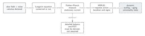
After a quench, the stochastic process may exhibit domain growth and aging rather than a stationary measure. Scaling then depends on the selected slow variables, conservation law, defects, initial condition, and quench protocol; detailed balance of the final bath does not restore time-translation invariance at finite waiting time. The diagram’s endpoint denotes tests for scaling or aging, not a universal exponent. It is schematic and not to scale.

The sections Domain-growth scaling, Defects and topology, and Aging observables give the text and equation equivalent of the nonstationary endpoint and its model dependence.

Checked curvature estimate

For a circular Model-A domain of radius $R$, mean curvature is proportional to $1/R$ and Allen–Cahn motion gives

$$\frac{dR}{dt}=-\frac{\lambda}{R}.$$

Thus

$$R^2(t)=R^2(0)-2\lambda t.$$

The collapse time scales as the initial radius squared, consistent with $L(t)\sim t^{1/2}$. This sharp-interface argument assumes a nonconserved scalar, isotropic tension, and negligible noise at the domain scale.

Failure tests

• Vary the quench depth, rate, initial correlations, and waiting-time origin.
• Demonstrate structure-factor collapse over an expanding $k$ and time window.
• Separate interface width, defect separation, and system size.
• Compare conserved and nonconserved dynamics explicitly.
• Test power laws against logarithmic and crossover forms.
• Measure two-time response rather than imposing equilibrium FDT.
• Repeat at larger volume to move finite-size saturation.

Exercise

If $L(t)\sim t^{1/2}$ and $f_C(y)\sim y^{-\lambda_C}$, what is the large-$t/t_w$ scaling of $C(t,t_w)$?

Solution

$L(t)/L(t_w)\sim(t/t_w)^{1/2}$, so $C(t,t_w)\sim(t/t_w)^{-\lambda_C/2}$ in the asymptotic aging regime.

Continue

This page is the stochastic nonequilibrium handoff. Compare any claimed scaling with the declared dynamic universality class and keep freeze-out, coarsening, aging, and eventual equilibration as separate regimes.

References

• Bray, A. J. (1994). “Theory of Phase-Ordering Kinetics.” Advances in Physics 43, 357–459. DOI.
• Cugliandolo, L. F. (2003). “Dynamics of Glassy Systems.” In Slow Relaxations and Nonequilibrium Dynamics in Condensed Matter, Les Houches Session LXXVII, 367–521. arXiv:cond-mat/0210312.