Convexity, Gauge Dependence, and Physical Phase Criteria

Physical phases are identified by thermodynamic limits, gauge-invariant operators, free-energy differences, correlation functions, and response—not by the coordinate of a gauge-fixed minimum. The exact Legendre effective potential is convex; barriers used for phase separation and nucleation belong to constrained, coarse-grained, or perturbatively continued objects whose domain must be stated.

Required background. Use thermal effective potentials for the perturbative construction and thermodynamic limits and phases for finite-volume qualifications.

Helpful background. Gauge and scale dependence of decay rates develops the corresponding semiclassical cancellation problem.

Why the exact potential is convex

For Euclidean source $J$ coupled linearly to an observable, $W[J]=\ln Z[J]$ has a positive-semidefinite second derivative equal to a connected covariance. Its Legendre–Fenchel transform $\Gamma[\phi]$ is therefore convex. At finite volume the equilibrium effective potential has one smooth minimum; in the infinite-volume coexistence limit it can develop a flat segment between pure-phase expectation values.

This does not erase interfaces or metastable dynamics. A constrained free energy fixes a spatial average, a Wilsonian action leaves infrared modes unintegrated, and a finite-resolution effective average action stops before full convexification. Such objects may retain barriers and supply useful interface or saddle data. Their barrier heights depend on scale, constraint, and volume and cannot be called exact equilibrium observables.

The Maxwell construction is the homogeneous thermodynamic reflection of phase separation: a mixed state realizes intermediate average order parameters with bulk free energy linear between pure phases, while the interfacial cost is subextensive. Nucleation instead studies a spatially inhomogeneous critical droplet in a metastable branch on times shorter than complete equilibration.

Gauge dependence and the Nielsen identity

For a gauge-fixed background $\varphi$ and gauge parameter $\xi$, the exact effective potential satisfies the identity derived in Nielsen 1975, pp. 177–180, of the form

$$\xi\frac{\partial V}{\partial\xi} +C(\varphi,\xi)\frac{\partial V}{\partial\varphi}=0.$$

Gauge variation is compensated by a change of field coordinate. Therefore the value of the exact potential at an exact stationary point is gauge independent, whereas the location $\varphi_{\min}$ generally is not. At finite order, extrema, $C$, derivative operators, and observables must be expanded in one power counting. Minimizing a truncated potential exactly can mix orders and leave spurious gauge dependence.

Physical phase criteria include equality of gauge-invariant pressure, discontinuities or susceptibilities of gauge-invariant operators, screening spectra, symmetry realization expressed by genuine observables, and nonperturbative finite-size scaling. In a gauge theory, a background Higgs coordinate can be a useful chart, but it is not an order parameter merely because two values are separated by a barrier.

The diagram below keeps three logically different objects apart: gauge- and scale-qualified coarse branches, the convex equilibrium Legendre object, and observable phase criteria. Its dashed lower branch is deliberately excluded from the equilibrium arrow.

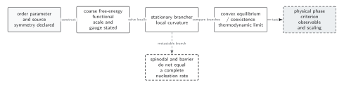
The exact equilibrium effective potential is convex, whereas a constrained, Wilsonian, or gauge-fixed coarse potential may retain local branches and barriers. Physical phase claims require gauge-invariant observables and controlled volume or scaling evidence; a barrier or spinodal is neither that evidence nor a complete rate. The diagram is schematic and not to scale.

The sections Why the exact potential is convex, Gauge dependence and the Nielsen identity, and A finite-volume check provide the text and equation equivalent; the uncertainty and validity table records the associated tests.

A finite-volume check

Suppose two pure phases have free-energy densities $f_1$ and $f_2$ and an extensive order parameter taking values $m_1,m_2$. At coexistence in a large box, a constrained average $m=(1-x)m_1+xm_2$ can be realized by volume fractions $1-x,x$. Its bulk free-energy density is

$$f(m)=(1-x)f_1+xf_2=f_1,$$

while an interface adds $O(L^{d-1})$ to the total free energy, or $O(1/L)$ to the density. Thus the infinite-volume effective potential is flat between $m_1$ and $m_2$ even though finite systems have an interface barrier. The scaling with $L$ distinguishes an interfacial cost from a bulk barrier.

Uncertainty and validity table

Evidence required at each stage from thermal landscape to transition completion

Stage	Computed object	Required checks	Principal failure mode	Strongest transferable claim
Landscape	Coarse-grained or perturbative functional with gradients	Symmetries, scale, invariants, regulator, derivative expansion	Treating a nonconvex model as the exact equilibrium potential	Candidate phases and interface scales in the stated description
Physical phase criterion	Free energies, gauge-invariant operators, susceptibilities	Thermodynamic limit, gauge/scale order counting, finite-size scaling	Inferring a phase from a gauge-fixed field coordinate	Coexistence or phase distinction for specified observables
Metastable regime	Local branch, Hessian, barrier, observation history	Finite volume, cooling rate, fluctuation scale, spinodal eigenvalue	Calling negative curvature nucleation or extrapolating beyond a spinodal	Nucleation-controlled or instability-controlled regime
Euclidean saddle	Periodic O(3), O(4), or less symmetric bounce action	Boundary conditions, one negative mode, zero modes, O(3)/O(4) crossover	Reporting $e^{-S_3/T}$ or $e^{-S_4}$ as a rate	Leading exponential suppression only
Statistical prefactor	Zero-mode Jacobian and regulated determinant ratio	Renormalization, collective coordinates, double counting, EFT matching	Using dimensional analysis in place of a determinant calculation	Equilibrium probability flux to the critical surface
Dynamical prefactor	Growth eigenvalue or real-time stochastic/kinetic response	Universality class, damping, conserved modes, scale separation	Assuming the Euclidean negative eigenvalue is a real-time rate	Nucleation rate in the validated dynamical theory
Wall propagation	Hydrodynamic branch and microscopic or calibrated friction	Frame, equation of state, wall thickness, stability, shocks, gauge/EFT validity	Assuming terminal velocity or ignoring competing branches	Growth law in the stated plasma regime
Percolation and completion	History integral for false-phase fraction with reheating and expansion	Rate history, wall law, overlap model, physical false-volume test	Equating one bubble per Hubble volume with completion	Converted fraction and completion status for the stated history
Downstream interface	Rates, wall profiles, thermodynamics, durations, and covariance	Units, conventions, evidence date, parameter range, uncertainty propagation	A baryogenesis or cosmology conclusion stronger than its inputs	Inputs to a separate downstream calculation

The later pages on metastability, nucleation, wall propagation, and completion use this table as their shared validity boundary.

Failure tests

• Identify the effective object and demonstrate its expected volume and coarse-graining dependence.
• Replace field-coordinate phase labels with measurable or gauge-invariant criteria.
• Check the Nielsen identity order by order, including derivative terms for inhomogeneous saddles.
• Compare finite-volume interface scaling with bulk free-energy scaling.
• Propagate gauge and scale variation through the final observable instead of stopping at the potential.

Exercise

Why can the value of $V$ at an exact extremum be gauge independent while the extremum position is gauge dependent?

Solution

At an extremum $\partial_\varphi V=0$, so the Nielsen identity gives $\partial_\xi V=0$. The compensating coefficient $C$ describes how the field coordinate changes with $\xi$; differentiating the stationarity condition shows that $\varphi_{\min}$ generally shifts. The invariant statement is the extremal value or a physical observable, not the coordinate.

Continue

Use metastability and spinodals to decide whether a branch decays through rare droplets or unstable growth. Carry this page’s table through every later inference.

References

• Fukuda, R., and Kugo, T. (1976). “Gauge Invariance in the Effective Action and Potential.” Physical Review D 13, 3469–3479. DOI.
• Nielsen, N. K. (1975). “On the Gauge Dependence of Spontaneous Symmetry Breaking in Gauge Theories.” Nuclear Physics B 101, 173–188. DOI.
• Patel, H. H., and Ramsey-Musolf, M. J. (2011). “Baryon Washout, Electroweak Phase Transition, and Perturbation Theory.” Journal of High Energy Physics 2011(07), 029. arXiv:1101.4665; DOI.