Nonlinear Response and Higher-Order Kubo Relations

Second- and higher-order response is expressed by causally ordered nested commutators plus source contacts. Unlike linear response, there are several inequivalent time-ordering sectors and several frequencies whose zero limits can approach the origin along different paths. A higher-order Kubo coefficient is meaningful only after those sectors, contacts, disconnected subtractions, frequency routing, symmetries, and constitutive-field conventions are all fixed.

Required background. Sources, linear response, and Kubo formulae fixes the source and retarded-sign convention. Sources and nonlinear response supplies closed-time-path differentiation and connected multipoint functions. Helpful background. Derivative expansion and tensor bases separates independent nonlinear constitutive structures.

The second-order causal kernel

Perturb the Hamiltonian by

$$H_f(t)=H_0-f_B(t)B-f_C(t)C,$$

with spatial labels suppressed. Expanding interaction-picture evolution to second order gives two causal sectors. A symmetric second-order kernel may be written

$$\begin{aligned} \mathcal R^{(2)}_{A;BC}(t;t_1,t_2) =-{}&\theta(t-t_1)\theta(t_1-t_2) \langle[[A(t),B(t_1)],C(t_2)]\rangle_c\\ -{}&\theta(t-t_2)\theta(t_2-t_1) \langle[[A(t),C(t_2)],B(t_1)]\rangle_c . \end{aligned}$$

Then

$$\delta^{(2)}\langle A(t)\rangle =\frac12\int dt_1dt_2\, \mathcal R^{(2)}_{A;BC}(t;t_1,t_2)f_B(t_1)f_C(t_2),$$

where the factor $1/2$ is omitted if one integrates over a single ordered domain instead. The nested-commutator sign follows from the same Hamiltonian convention that gives $\mathcal R^{(1)}=-G_R$. The subscript $c$ removes disconnected equilibrium pieces when the response is derived from $W=-i\log Z$.

The formula is causal but not a single ordinary retarded three-point function: exchanging the two source insertions changes the ordering sector. At order $n$ there are $n!$ sectors before symmetries are used. The nested-commutator expansion originates in the general response construction Kubo 1957, §§2–3, is standard in nonlinear spectroscopy Mukamel 1995, chs. 5–6, and is packaged by closed-time-path $r/a$ differentiation without losing causal information Crossley, Glorioso, and Liu 2017, §§2–3, Open PDF.

Contacts proliferate beyond linear order

If the observable or source-coupled operator depends on $f$, differentiation gives terms such as

$$\left\langle\frac{\delta^2 A_f}{\delta f_B\delta f_C}\right\rangle, \qquad \left\langle \frac{\delta A_f}{\delta f_B}\,C \right\rangle_c, \qquad \left\langle A\,\frac{\delta B_f}{\delta f_C} \right\rangle_c.$$

They are localized when insertion times coincide and are fixed by the nonlinear source functional. Gauge and diffeomorphism Ward identities generally require them. A three-point correlator of the zero-source operators is therefore insufficient for a second-order conductivity or metric response.

Local field redefinitions create a related but distinct issue. A nonlinear constitutive coefficient attached to $u^\mu$, $T$, or $\mu$ may change when those hydrodynamic variables are redefined. The Kubo relation must project onto a frame-invariant observable or state the chosen frame and operator basis. A response function is observable; an individual coefficient in a redundant constitutive basis need not be.

Frequency routing and zero-limit paths

Time-translation invariance imposes frequency conservation. With output frequency $\omega$ and two inputs,

$$\omega=\omega_1+\omega_2.$$

A dc rectification experiment takes $\omega_1=\Omega$ and $\omega_2=-\Omega$ before $\Omega\to0$. A second-harmonic experiment takes $\omega_1=\omega_2=\Omega$ and observes $2\Omega$. A quasistatic nonlinear susceptibility sends both frequencies to zero without first imposing a homogeneous transport geometry. These are different paths through the same multipoint function.

Hydrodynamic denominators such as $(-i\omega_a+Dk_a^2)^{-1}$ make the paths noncommuting. One must also state whether the combined output momentum is taken to zero before or after each input momentum. Analytic continuation from Euclidean three-point data is correspondingly multivariable; continuing only the total Matsubara frequency does not determine every real-time causal sector.

Symmetry before calculation

Spatial, internal, and antiunitary symmetries reduce the tensor basis before any limit is taken. For example,

$$J_i^{(2)}=\chi^{(2)}_{ijk}E_jE_k.$$

In a centrosymmetric equilibrium state, inversion sends $J_i\mapsto-J_i$ and $E_jE_k\mapsto E_jE_k$, so $\chi^{(2)}_{ijk}=0$. A nonzero quadratic electric response then diagnoses broken inversion, a nonequilibrium background, a boundary, or a misidentified contact—not merely “nonlinearity.”

Time reversal gives generalized Onsager relations, but it maps a causal multipoint function to a reversed, generally advanced ordering with the product of operator parities. It does not imply naive symmetry under every index permutation. Detailed balance or dynamical KMS supplies the precise thermal relation Wang and Heinz 2002, §§II–III, Open PDF.

A reproducible higher-order Kubo relation

Before quoting a nonlinear coefficient, record:

1. the complete source functional through the required order;
2. the connected causal sectors and Fourier routing;
3. all coincident-source contacts and equilibrium subtractions;
4. the tensor projector, symmetry sector, and operator normalization;
5. the path by which all frequencies and momenta approach zero;
6. the hydrodynamic frame or frame-invariant combination;
7. the spectral or real-time resolution needed to distinguish the claimed coefficient.

These declarations are the nonlinear analogue of the transport-extraction covariance reference.

The response box below explicitly includes both linear and nonlinear functions. Inspect how the same subsequent gates—contacts, zero-limit paths, spectral constraints, covariance, and resolution—remain necessary when a nested commutator carries several frequencies.

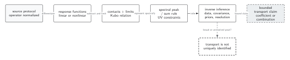
Higher-order response begins with repeated differentiation of the complete source functional, not with a guessed nested commutator alone. Coincident-source contacts, causal sectors, frequency routing, symmetry projections, and the multidimensional zero-limit path must be fixed before inference. The diagram is schematic and suppresses the branching time orderings of a nonlinear kernel.

In text: enumerate the causal permutations, add every local derivative of the source-coupled operator, impose spatial and antiunitary symmetries, and declare how all external frequencies and momenta vanish. Only combinations identifiable under the resulting multipoint forward kernel may be reported.

Exercise: inversion forbids quadratic conductivity

Prove that an isotropic centrosymmetric medium has no homogeneous second-order electric conductivity at zero magnetic field. Which assumption can be relaxed to allow one?

Solution

The most general homogeneous quadratic term is $J_i=\chi^{(2)}_{ijk}E_jE_k$. Under inversion, both $J_i$ and $E_i$ are polar vectors, so the left side changes sign while the product $E_jE_k$ does not. Invariance of the equilibrium state requires

$$-J_i=\chi^{(2)}_{ijk}E_jE_k=J_i,$$

for arbitrary fields; hence $\chi^{(2)}_{ijk}=0$. Broken inversion in the material, a boundary or interface, a parity-odd background such as a magnetic field, spatial gradients, or an explicitly driven nonequilibrium state can evade the argument. Which possibility applies must be stated before interpreting a measured quadratic signal.

References

• Crossley, Michael, Paolo Glorioso, and Hong Liu. 2017. “Effective Field Theory of Dissipative Fluids.” Journal of High Energy Physics 2017 (9): 095. DOI. Open PDF.
• Kubo, Ryogo. 1957. “Statistical-Mechanical Theory of Irreversible Processes. I. General Theory and Simple Applications to Magnetic and Conduction Problems.” Journal of the Physical Society of Japan 12 (6): 570–586. DOI.
• Mukamel, Shaul. 1995. Principles of Nonlinear Optical Spectroscopy. New York: Oxford University Press. Publisher.
• Wang, Enke, and Ulrich Heinz. 2002. “A Generalized Fluctuation–Dissipation Theorem for Nonlinear Response Functions.” Physical Review D 66 (2): 025008. DOI. Open PDF.

Spectral Functions and Transport Peaks interprets the one-frequency singularities that already complicate linear response. Transport Extraction, Inverse Problems, and Error Budgets explains why multipoint analytic continuation is even less identifiable without strong forward information.