Exact Euclidean–Real-Time Analytic Continuation

Exact Euclidean thermal data determine a retarded correlator when they are boundary values of a function with the required analyticity, growth, spectral, and subtraction properties. Under the Baym–Mermin conditions, the full Matsubara sequence selects the physical analytic continuation. A finite noisy subset does not: infinitely many functions fit those samples, and continuation amplifies their poorly constrained directions.

The classic uniqueness conditions separating Matsubara data from arbitrary interpolants are given by Baym and Mermin 1961, pp. 232–234.

Required background. Thermal Propagators and Spectral Representations gives the common spectral representation. Branches, Sheets, Analytic Continuation, and Monodromy supplies path and branch control. Helpful background. Thermal Spectral Positivity and Sum Rules gives channel constraints that can restrict, but not replace, analytic input.

Analytic function and physical boundary values

For a neutral bosonic channel, define the complex-energy function

$$\mathcal G(z,\mathbf p)= \int\frac{\mathrm d\omega'}{2\pi} \frac{\rho(\omega',\mathbf p)}{z-\omega'}$$

after the subtractions required by its ultraviolet behavior. It is analytic for $z$ off the real-axis singular support. The physical boundary values are

$$G_R(\omega,\mathbf p)=\mathcal G(\omega+i0,\mathbf p), \qquad G_A(\omega,\mathbf p)=\mathcal G(\omega-i0,\mathbf p).$$

With the Euclidean convention of the preceding page, for nonzero Matsubara frequencies,

$$G_E(i\omega_n,\mathbf p)=-\mathcal G(i\omega_n,\mathbf p).$$

Thus the retarded mnemonic continuation starts from the positive-frequency sequence,

$$G_R(\omega,\mathbf p) =-G_E(i\omega_n\to\omega+i0,\mathbf p), \qquad n>0,$$

but only after $G_E$ has been identified as the restriction of the eligible analytic function. Negative Matsubara frequencies approach the lower-half-plane branch, and a zero mode on a nonanalytic origin requires a separately specified static limit. Replacing a discrete label inside an arbitrary interpolation is not analytic continuation.

A solvable round trip

For a free scalar,

$$G_E(i\omega_n,\mathbf p) =\frac1{\omega_n^2+E_{\mathbf p}^2}.$$

The meromorphic function

$$\mathcal G(z,\mathbf p)=\frac1{z^2-E_{\mathbf p}^2}$$

satisfies $G_E(i\omega_n)=-\mathcal G(i\omega_n)$ and decays as $z^{-2}$. Taking the upper boundary value yields

$$G_R(\omega,\mathbf p) =\frac1{(\omega+i0)^2-E_{\mathbf p}^2}.$$

The poles lie below the real axis in the causal factorization, and the resulting spectral discontinuity matches the canonical commutator. These pole, decay, and sum-rule checks identify the physical continuation rather than merely a curve through discrete points.

Why the full sequence needs growth conditions

Values at $z=i2\pi nT$ do not determine an arbitrary analytic function. One may add a function containing $\sinh(\beta z/2)$, which vanishes at every bosonic Matsubara point, without changing the samples. Such additions generally violate the physical growth, analyticity, or spectral conditions. Baym and Mermin showed that imposing the thermal boundary structure and suitable behavior at complex infinity selects the physical continuation Baym and Mermin 1961.

If the correlator grows polynomially, first write a subtracted dispersion relation,

$$\mathcal G(z)=P_{N-1}(z) +z^N\int\frac{\mathrm d\omega'}{2\pi} \frac{\rho(\omega')}{(\omega')^N(z-\omega')}.$$

The subtraction polynomial $P_{N-1}$ is extra data fixed by contact terms or renormalization conditions. Spectral discontinuities do not determine it.

Exact uniqueness versus numerical stability

Uniqueness and stability are logically independent. Even when exact continuum $G_E(\tau)$ uniquely fixes $\rho$, the kernel

$$G_E(\tau)=\int\frac{\mathrm d\omega}{2\pi} \frac{e^{-\omega\tau}}{1-e^{-\beta\omega}}\rho(\omega)$$

smooths spectral structure. Its singular values decay rapidly after discretization. Small Euclidean perturbations can therefore correspond to large changes in a narrow real-time feature. Exact analytic continuation is a theorem about perfect data in a constrained function class; reconstruction is an inference problem with resolution and covariance.

Continuation checklist

• Name the analytic variable, domain, cuts, poles, and boundary side.
• State KMS periodicity, operator grading, and any chemical twist.
• Derive the ultraviolet growth and number of subtractions.
• Include contact polynomials not encoded by the spectral discontinuity.
• Demonstrate that the complete exact data, not a chosen interpolation, satisfy the uniqueness hypotheses.
• Round-trip the continued function back to all Matsubara values.
• Check a commutator sum rule or known solvable limit.
• If the data are finite or noisy, stop calling the operation exact and use the inference contract on the next page.

The shared equilibrium convention table keeps exact continuation distinct from inverse reconstruction.

The schematic below organizes the relationships used on this page. Inspect it with this question in mind: What connects thermal correlators, spectral densities, exact continuation, and finite-data reconstruction?

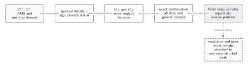
KMS and the commutator determine compatible Euclidean and retarded representations; exact analytic continuation is unique under its hypotheses, whereas reconstructing a spectrum from finite noisy data is an ill-posed inference problem. Solid connections show the primary relation; dashed outlines or arrows mark qualifications and failure boundaries. The diagram is schematic and not to scale.

The surrounding discussion supplies the relevant equations and checks in text form; the figure is a navigational summary.

Exercise

Why is adding $c\sinh(\beta z/2)e^{-z^2/\Lambda^2}$ not automatically an allowed alternative continuation, even though it vanishes at all bosonic Matsubara points?

Solution

Matching the discrete points is only one condition. The added entire function has direction-dependent exponential growth because $e^{-z^2/\Lambda^2}$ grows along imaginary directions, and it need not admit the required spectral representation, causality, or ultraviolet bounds. Physical uniqueness theorems exclude alternatives by the complete analytic and growth class, not by the samples alone.

References

• Baym, Gordon, and N. David Mermin. “Determination of Thermodynamic Green’s Functions.” Journal of Mathematical Physics 2, no. 2 (1961): 232–234. doi:10.1063/1.1703704.
• Cuniberti, Gianaurelio, Erik De Micheli, and Giovanni A. Viano. “Reconstructing the Thermal Green Functions at Real Times from Those at Imaginary Times.” Communications in Mathematical Physics 216 (2001): 59–83. doi:10.1007/s002200000317.
• Evans, T. S. “What Is Being Calculated with Thermal Field Theory?” Nuclear Physics B 374, no. 2 (1992): 340–370. doi:10.1016/0550-3213(92)90355-M.