2PI Effective Actions and Conserving Truncations

A 2PI truncation closes the two-time equations by deriving the self-energy from one functional of the full propagator. If the truncated functional preserves a continuous global symmetry, the resulting self-consistent solution obeys the associated macroscopic conservation law. That theorem does not imply exact Ward–Takahashi identities, gauge-parameter independence, crossing symmetry, or quantitative accuracy.

Required background. Use two-time self-energies for the contour notation and 2PI and nPI effective actions for Legendre transforms and skeleton counting.

Helpful background. Operator mixing and renormalization matrices clarifies why a self-consistent composite functional generally needs more counterterm conditions than a one-loop 1PI calculation.

Stationarity generates the closure

For vanishing one-point function, the bosonic two-particle-irreducible action may be written

$$\Gamma[G]=\frac{i}{2}\operatorname{Tr}\ln G^{-1} +\frac{i}{2}\operatorname{Tr}(G_0^{-1}G-1) +\Gamma_2[G]+\Gamma_{\mathrm{ct}}[G].$$

$\Gamma_2$ is the sum of closed 2PI skeletons built with full $G$ and bare vertices. Stationarity,

$$\frac{\delta\Gamma}{\delta G}=0, \qquad \Sigma(x,y)=2i\frac{\delta(\Gamma_2+\Gamma_{\mathrm{ct}})}{\delta G(y,x)},$$

produces the Dyson equation. Loop, coupling, $1/N$, or nPI counting defines the approximation; saying merely “two-loop 2PI” is incomplete unless the retained skeletons and counterterms are listed.

As a concrete scalar example, for $\mathcal L_{\mathrm{int}}=-\lambda\phi^4/4!$, the lowest nonlocal 2PI skeleton is the three-loop setting-sun diagram. Its functional derivative produces a self-energy cubic in the full propagator, and therefore nonlocal $\Sigma_F$ and $\Sigma_\rho$. The two-loop double-bubble gives a local, self-consistent mass but no scattering width. This difference is a simple check: a claimed damping rate cannot arise from a closure whose self-energy is purely local.

What “conserving” proves

Baym’s theorem applies when the approximation is $\Phi$-derivable: the same invariant truncated functional generates both the equations and the current or stress tensor. Infinitesimal translations then imply conservation of the corresponding self-consistent energy–momentum tensor, while a global internal symmetry implies its Noether current. Conservation is lost if one mixes propagators and self-energies from different truncations, truncates memory inconsistently, or changes the numerical equation without changing the conserved functional.

The theorem has sharp limits. Variational vertices obtained directly from $\delta\Gamma/\delta G$ and resummed external vertices obtained from further functional derivatives need not coincide at finite truncation. Consequently exact crossing relations and Ward–Takahashi identities can fail. In gauge theories, conserving a global charge does not cancel gauge-parameter dependence or restore Slavnov–Taylor identities. Arrizabalaga and Smit 2002 exhibit the controlled but nonzero gauge dependence of truncated 2PI approximations. A gauge calculation must therefore specify gauge fixing, power counting, vertex completion, and residual identity tests.

Renormalization and initial-time compatibility

Self-consistency resums infinitely many ordinary diagrams, so counterterms must be fixed at the level of the truncated integral equations. Vacuum subdivergences, medium-independent counterterms, and the distinction between variational and resummed vertices must be treated consistently. Renormalizing a single mass equation while leaving the four-point kernel unrenormalized is insufficient; systematic constructions are given by van Hees and Knoll 2002.

At finite $t_0$, a Gaussian initial state whose ultraviolet correlations do not approach the renormalized vacuum can generate uncancelled boundary singularities. One must either prepare the interacting state, include suitable initial correlation vertices and boundary counterterms, or demonstrate cutoff-stable observables after an explicitly controlled switch-on. Initial-time transients are not automatically physical relaxation.

The dashed branch in the hierarchy marks the central limitation of a $\Phi$-derivable closure. Symmetry-generated global conservation laws and gauge-theory Ward identities are different claims and require different checks.

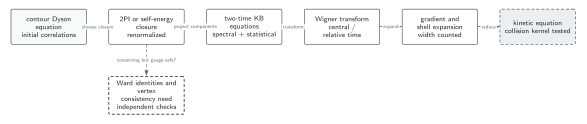
A self-consistent 2PI truncation generated from a symmetry-respecting $\Phi$ functional can conserve the associated global Noether charges and energy–momentum under consistent evolution. That result does not automatically preserve gauge Ward or Slavnov–Taylor identities, vertex consistency, positivity, or renormalized initial-time behavior. The dashed branch requires those independent tests before any kinetic reduction. The diagram is schematic and not to scale.

The sections Stationarity generates the closure, What “conserving” proves, and Renormalization and initial-time compatibility provide the text and equation equivalent; the following table lists the independent numerical tests.

Conservation and numerical validation matrix

Minimum evidence needed to interpret a truncated two-time evolution

Claim	Required record	Primary check	Failure signal	Strongest justified conclusion
Self-energy closure	All retained skeletons, counting parameter, propagator and vertex definitions	Differentiate the stated $\Gamma_2$ and recover every term in $\Sigma$	A damping term has no parent skeleton or a local closure produces a width	Solution of the named truncation only
Initial correlations	Density matrix or boundary cumulants, preparation time, UV tail	Vary preparation and include the first omitted cumulant	Persistent initial slip or cutoff-dependent early-time spike	Evolution for the specified preparation
Renormalization	Regulator, counterterms, renormalization conditions, vacuum subtraction	Cutoff variation at fixed renormalized parameters	Observable drift with cutoff or initial time	Regulator-independent result within the tested window
Spectral normalization	Equal-time commutator and frequency-moment convention	$\rho(t,t)=0$ and $\partial_t\rho(t,t')|_{t=t'}=1$ for every mode	Sum-rule drift or loss of antisymmetry	Canonical two-point normalization
Conservation	Explicit truncated energy or charge functional	Drift versus timestep, grid, and memory window	Drift plateaus under solver refinement but changes with memory cutoff	Macroscopic conservation of the stated $\Phi$-derivable closure
Ward or gauge consistency	Gauge fixing, variational and resummed vertices, identity residuals	Gauge-parameter and Ward–Takahashi residual study	Conserved energy but gauge-dependent observable	No stronger than the measured residuals permit
Memory reduction	Full and truncated kernels, cutoff rule, tail estimate	Increase the memory window through the longest correlation time	Late-time rate or energy changes with the window	Controlled history truncation over the tested duration
Time and space discretization	Integrator, $\Delta t$, volume, grid spacing, solver tolerance	Independent refinement and observed convergence order	Only the combined refinement looks stable	Discrete convergence, not continuum closure accuracy
Gradient or quasiparticle reduction	Wigner window, gradient order, width and shell assumptions	Compare with unreduced two-time evolution	Agreement only after fitting an effective relaxation time	Kinetic reduction in the demonstrated regime
Independent benchmark	Free, large-$N$, exact-diagonalization, or kinetic control with matched inputs	Blind comparison of conserved and nonconserved observables	Visual agreement but incompatible normalization or preparation	Agreement for the matched benchmark and observables

This matrix is used again for initial correlations, memory kernels, and numerical validation.

Exercise

Suppose $\Gamma_2[G]$ is invariant under a global transformation $G(x,y)\mapsto U G(x,y)U^{-1}$, but a numerical code evaluates $\Sigma[G]$ with a memory cutoff and the energy with the uncut functional. Does Baym’s conservation theorem apply?

Solution

No. The implemented equation is no longer the stationary equation of the functional used to define the energy. The symmetry of the formal $\Gamma_2$ is insufficient; the discretized, memory-truncated evolution and monitored charge must arise from a mutually consistent approximation. Conservation may still be approximate, but its residual must be measured and shown to converge as the memory window and timestep are refined.

Continue

Derive the causal component equations on Kadanoff–Baym evolution. Before interpreting a run, apply the matrix above and the detailed numerical validation protocol.

References

• Arrizabalaga, A., and Smit, J. (2002). “Gauge-Fixing Dependence of $\Phi$-Derivable Approximations.” Physical Review D 66, 065014. arXiv:hep-ph/0207044; DOI.
• Baym, G. (1962). “Self-Consistent Approximations in Many-Body Systems.” Physical Review 127, 1391–1401. DOI.
• Cornwall, J. M., Jackiw, R., and Tomboulis, E. (1974). “Effective Action for Composite Operators.” Physical Review D 10, 2428–2445. DOI.
• van Hees, H., and Knoll, J. (2002). “Renormalization in Self-Consistent Approximation Schemes at Finite Temperature. I: Theory.” Physical Review D 65, 105005. arXiv:hep-ph/0111193; DOI.