Kadanoff–Baym Evolution Equations

The Kadanoff–Baym equations are the exact contour Dyson equation resolved into two causal equations: one propagates the state-dependent statistical correlator $F$, the other propagates the canonically normalized spectral correlator $\rho$; the $F/\rho$ form is derived in Berges 2004, § 3.4. A practical evolution becomes approximate only when one chooses a self-energy closure, initial data, regulator, or numerical discretization.

Required background. Two-time Green functions and self-energies fixes the contour decomposition used below.

Helpful background. 2PI truncations generate self-consistent kernels, while causal and statistical propagators explain the independent initial data.

Component equations and causal limits

For a spatially homogeneous real scalar field, write $F_{\mathbf p}(t,t')$ and $\rho_{\mathbf p}(t,t')$ and absorb the local self-energy into

$$\Omega_{\mathbf p}^2(t)=\mathbf p^2+m^2+\Sigma^{(0)}(t).$$

With $F=\tfrac12\langle\{\phi,\phi\}\rangle$ and $\rho=i\langle[\phi,\phi]\rangle$, the contour convolution gives

$$\begin{aligned} [\partial_t^2+\Omega_{\mathbf p}^2(t)]F_{\mathbf p}(t,t') ={}&-\int_{t_0}^{t}du\,\Sigma_{\rho,\mathbf p}(t,u)F_{\mathbf p}(u,t')\\ &+\int_{t_0}^{t'}du\,\Sigma_{F,\mathbf p}(t,u)\rho_{\mathbf p}(u,t'),\\[3pt] [\partial_t^2+\Omega_{\mathbf p}^2(t)]\rho_{\mathbf p}(t,t') ={}&-\int_{t'}^{t}du\,\Sigma_{\rho,\mathbf p}(t,u)\rho_{\mathbf p}(u,t'). \end{aligned}$$

Spatial convolutions are implicit if translation invariance is absent. The upper limits encode causality. In particular, the spectral equation at $(t,t')$ needs only the strip between $t'$ and $t$, whereas the statistical equation remembers the preparation time through both kernels. Replacing either limit by infinity assumes stationarity and erases the initial-value problem.

The adjoint equations obtained by differentiating in $t'$ are not optional: together with $F(t,t')=F(t',t)$ and $\rho(t,t')=-\rho(t',t)$ they provide strong implementation checks. For bosons the canonical conditions are

$$\rho_{\mathbf p}(t,t)=0, \qquad \partial_t\rho_{\mathbf p}(t,t')\big|_{t=t'}=1, \qquad \partial_t\partial_{t'}\rho_{\mathbf p}(t,t')\big|_{t=t'}=0.$$

$F(t_0,t_0)$ and its first derivatives specify a Gaussian initial covariance subject to the uncertainty principle. Non-Gaussian initial cumulants add boundary terms treated on the initial-correlations page.

How the equations follow from contour ordering

The key identity is the contour decomposition

$$A_{\mathcal C}=A_F-\frac{i}{2}\operatorname{sgn}_{\mathcal C}A_\rho$$

for both $G$ and the nonlocal self-energy. Multiplying $\Sigma_{\mathcal C}G_{\mathcal C}$, collecting its symmetric and antisymmetric parts, and splitting the forward and backward contour segments yields the two real-time integrals above. No gradient expansion, on-shell delta function, or molecular-chaos assumption appears. Those are later reductions, so a derivation that writes a Boltzmann collision term at this stage has skipped essential hypotheses.

The equation is closed only after specifying $\Sigma_F[F,\rho]$ and $\Sigma_\rho[F,\rho]$. A perturbative self-energy evaluated with free propagators and then inserted indefinitely is generally not the same approximation as a stationary 2PI truncation; their conservation properties differ.

The hierarchy makes clear what closes the displayed evolution: a declared and renormalized self-energy functional, together with compatible initial data. The causal integration limits follow from contour projection; they do not make the closure exact.

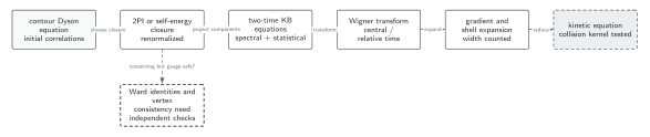
The Kadanoff–Baym equations are the spectral and statistical components of the contour Dyson equation for the chosen self-energy and initial correlations. Their finite-time memory limits encode causality and preserve two-time information. Wigner transformation, gradient truncation, shell projection, and Markovization are later reductions, not hidden steps in these equations. The diagram is schematic and not to scale.

The sections Component equations and causal limits and How the equations follow from contour ordering give the explicit text and equation equivalent of the central Kadanoff–Baym box.

Checked oscillator limit

Set $\Sigma_F=\Sigma_\rho=0$ and $\Omega(t)=\omega$. For a Gaussian state,

$$F(t,t')=\frac{n+\tfrac12}{\omega}\cos[\omega(t-t')], \qquad \rho(t,t')=\frac{\sin[\omega(t-t')]}{\omega}.$$

Direct differentiation annihilates both functions, and the sine solution gives the canonical derivative $1$. If a numerical code fails this zero-self-energy test at machine precision up to the integrator’s expected global error, its interacting damping cannot be trusted.

For a time-dependent local frequency but no nonlocal self-energy, the Wronskian of two mode solutions preserves the spectral normalization. This tests a mass-quench implementation independently of collision integrals.

Failure tests

1. Signs and limits. Turn off $\Sigma_F$ while keeping a test $\Sigma_\rho$ and compare the component equation with direct contour convolution. A branch-sign error often preserves symmetry but violates the equal-time derivative.
2. Closure. Differentiate the stated 2PI functional and match every kernel term. A hand-added relaxation term forfeits the conserving theorem.
3. Initial surface. Vary $t_0$ while holding the physical preparation fixed. Uncontrolled $t_0$ dependence signals missing correlations or boundary renormalization.
4. No hidden kinetics. Compare the full two-time solution with any Wigner or quasiparticle reduction while varying the gradient order and spectral width.

The chapter’s conservation and numerical validation matrix records the evidence required for each of these claims.

Exercise

Use antisymmetry of $\rho$ to show that its equation preserves $\rho(t,t)=0$. Why does this not by itself guarantee the derivative sum rule?

Solution

At equal times the integration interval in the spectral equation collapses, so the right-hand side vanishes; antisymmetric initial data therefore retain zero diagonal value. The derivative condition comes from the canonical commutator and fixes the Wronskian. A discretization can keep an antisymmetric matrix while slowly changing its near-diagonal slope, so the derivative sum rule must be monitored separately.

Continue

Add correlated preparation through initial boundary terms, test history reduction with memory kernels, and use numerical validation before drawing physical conclusions.

References

• Aarts, G., and Berges, J. (2001). “Nonequilibrium Time Evolution of the Spectral Function in Quantum Field Theory.” Physical Review D 64, 105010. arXiv:hep-ph/0103049; DOI.
• Berges, J. (2004). “Introduction to Nonequilibrium Quantum Field Theory.” AIP Conference Proceedings 739, 3–62. arXiv:hep-ph/0409233; DOI.
• Danielewicz, P. (1984). “Quantum Theory of Nonequilibrium Processes, I.” Annals of Physics 152, 239–304. DOI.