Detailed Balance and Fluctuation–Dissipation

Detailed balance is stronger than stationarity. For variables even under time reversal and no magnetic or other time-odd background, it is equivalent to vanishing stationary probability current. It implies an equilibrium time-reversal symmetry and fluctuation–dissipation relations. A steady circulating current violates detailed balance even if the stationary density is exactly Gibbs shaped.

Required background. Use Fokker–Planck probability current and the MSRJD response functional.

Helpful background. Onsager reciprocity and entropy production gives the macroscopic near-equilibrium consequences.

Probability-current criterion

For an Itô diffusion with current

$$J_i=a_iP-\frac12\partial_j(D_{ij}P),$$

a stationary density satisfies $\partial_iJ_i=0$. For purely even variables, detailed balance requires $J_i^{\mathrm{st}}=0$ under suitable boundary conditions. This makes the generator self-adjoint after weighting by $P_{\mathrm{st}}$ and yields equality of forward and time-reversed path probabilities.

Variables such as momentum are odd under time reversal. Hamiltonian reversible currents need not vanish; detailed balance instead reverses their sign while the irreversible current vanishes. Magnetic fields, rotation, and other time-odd parameters must also be reversed in the comparison. Applying the even-variable zero-current test to underdamped dynamics incorrectly labels equilibrium phase-space circulation as dissipation.

Model-A fluctuation–dissipation relation

For a Gaussian mode, the classical response–correlation relation descending from Kubo 1957, §§ 2–3 is seen from

$$C_k(t)=\langle\phi_{\mathbf k}(t)\phi_{-\mathbf k}(0)\rangle =\frac{T}{r+k^2}e^{-\Gamma(r+k^2)|t|},$$

and response to $-\!h\phi$ in the free energy,

$$R_k(t)=\Gamma\theta(t)e^{-\Gamma(r+k^2)t}.$$

They obey

$$R_k(t)=-\frac{1}{T}\theta(t)\frac{dC_k(t)}{dt}.$$

This classical FDT follows from detailed balance and the declared source normalization. Fourier transformation gives the equivalent relation between $C(\omega)$ and the dissipative part of the response. A different mobility convention moves factors of $\Gamma$ but cannot change the physical finite-difference response.

The dashed branch in the schematic is deliberately a question—“equilibrium?”—rather than an automatic arrow. Detailed balance is established by the probability current or the equivalent stochastic symmetry, and only then yields the equilibrium fluctuation–dissipation relation.

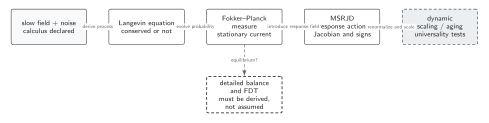
A stationary measure lies on the equilibrium branch only when the appropriate stationary probability current vanishes, or an equivalent detailed-balance condition holds. Under that condition response and fluctuations obey FDT. A circulating steady current provides the counterexample: stationarity can persist while detailed balance, the equilibrium FDT, and time-reversal symmetry fail. The diagram is schematic and not to scale.

The sections Probability-current criterion, Model-A fluctuation–dissipation relation, and Stationary nonequilibrium counterexample give the text and equation equivalent of the dashed branch.

Stationary nonequilibrium counterexample

Consider a two-dimensional Ornstein–Uhlenbeck process

$$\dot{\mathbf x} =-\gamma\mathbf x+\Omega\,\mathbf R\mathbf x+\boldsymbol\xi, \qquad \mathbf R= \begin{pmatrix}0&-1\\1&0\end{pmatrix},$$

with isotropic noise $2D$. The stationary density is the same Gaussian $P\propto e^{-\gamma|\mathbf x|^2/(2D)}$ as for $\Omega=0$, but

$$\mathbf J_{\mathrm{st}}=\Omega\,\mathbf R\mathbf x\,P_{\mathrm{st}}\ne0.$$

The current is divergence free and circulates along density contours. Stationarity therefore does not imply detailed balance; response contains a rotational component not fixed by the equilibrium scalar covariance.

Entropy production and stochastic symmetry

For overdamped diffusion with positive $D$, the irreversible entropy production is schematically

$$\dot S_{\mathrm{tot}} =\int dx\,\frac{J_{\mathrm{irr}}^TD^{-1}J_{\mathrm{irr}}}{P}\ge0.$$

It vanishes under detailed balance. In MSRJD language, equilibrium time reversal transforms both $\phi$ and the response field, shifting the latter by a term proportional to $\delta\mathcal F/\delta\phi$. Boundary terms encode the Gibbs weight. Multiplicative noise changes this transformation through its convention and Jacobian.

Failure tests

• Separate reversible and irreversible currents using correct time-reversal parities.
• Reverse time-odd external fields in the comparison process.
• Test probability current, path-weight symmetry, and FDT independently.
• Include boundary currents and multiplicative-noise drift.
• Avoid assigning an effective temperature from one observable in a driven state.
• Verify zero entropy production within numerical resolution and regulator control.

Exercise

Show that the rotational current in the counterexample is divergence free.

Solution

$\nabla\cdot(\mathbf R\mathbf x)=\operatorname{tr}\mathbf R=0$. The Gaussian gradient is parallel to $\mathbf x$, while $\mathbf R\mathbf x$ is perpendicular, so $(\mathbf R\mathbf x)\cdot\nabla P=0$. Hence $\nabla\cdot\mathbf J_{\mathrm{st}}=0$ despite $\mathbf J_{\mathrm{st}}\ne0$.

Continue

Use detailed balance to classify equilibrium models on dynamic universality classes and identify its modifications on multiplicative, colored, and conserved noise.

References

• Callen, H. B., and Welton, T. A. (1951). “Irreversibility and Generalized Noise.” Physical Review 83, 34–40. DOI.
• Kubo, R. (1957). “Statistical-Mechanical Theory of Irreversible Processes. I.” Journal of the Physical Society of Japan 12, 570–586. DOI.