

Hydrodynamic Fluctuations and Noise
Thermal hydrodynamic fluctuations are stochastic fluctuations of the same conserved densities and currents that appear in deterministic constitutive relations. In equilibrium, fluctuation–dissipation fixes their two-point kernel from the dissipative transport matrix. White Gaussian noise is only the leading Markovian, classical, coarse-grained limit; nonlinear variables, causal completions, quantum frequencies, and finite regulators generally produce multiplicative, colored, non-Gaussian, or bilocal structures.
Required background. KMS Relations and Fluctuation–Dissipation fixes the equilibrium noise–response relation. Relativistic Dissipative Hydrodynamics supplies the transport coefficients.
Helpful background. Strong Hyperbolicity, Stability, and Causal Propagation and BDNK First-Order Causal Hydrodynamics separate causal PDE structure from infrared transport. Multiplicative, Colored, and Conserved Noise develops stochastic prescriptions.
Conserved diffusion with matched noise
Section titled “Conserved diffusion with matched noise”Let be one charge density, its static susceptibility, and its conductivity. At fixed temperature,
The continuity equation becomes
In the local classical equilibrium and Markov limits, fluctuation–dissipation requires
Solving in Fourier space gives the symmetric density correlator
Its equal-time integral is the independent check:
The same diffusion normalization and its relation to retarded response are derived in Kovtun 2012, §§2.3 and 3.1, Open PDF.
The noise is a current, rather than an additive density source, so exact conservation survives realization by realization. Landau and Lifshitz give the corresponding stochastic stress tensor; in a local rest frame its shear and bulk covariance is fixed by and with the same tensor projectors as the viscous stress Landau and Lifshitz 1987, §XVII, pp. 537–545.
When white Gaussian noise is justified
Section titled “When white Gaussian noise is justified”The delta functions approximate a microscopic kernel whose correlation time and length are unresolved. They require
and a cell containing enough microscopic degrees of freedom for Gaussian closure. The continuum variance at one point diverges: is not an observable. A lattice spacing, smoothing kernel, or momentum cutoff must be declared, and bare thermodynamic and transport parameters then depend on it.
If , , or the hydrodynamic measure depends on the fluctuating fields, the noise is multiplicative. Itô, Stratonovich, kinetic, or a time-symmetric prescription changes drift and Jacobian terms. The prescription is part of the theory, not a numerical option. Non-Gaussian cumulants arise beyond the quadratic effective action and are constrained, but not generally fixed, by equilibrium symmetry.
At quantum frequencies the classical factor is replaced by the KMS frequency kernel. The symmetrized noise is colored even in equilibrium, schematically through ; the white expression is its limit.
Causal formulations change the kernel
Section titled “Causal formulations change the kernel”Consider a relaxing current,
White forcing of this enlarged Markov system produces an effective current spectrum proportional to
after the transient current is eliminated. Thus a local differential representation can become colored and temporally nonlocal in a density-only representation. Noise variables, response kernel, and initial covariances must be transformed together.
This point is sharper for BDNK. A linear stochastic BDNK construction generally has a bilocal Martin–Siggia–Rose action and nonwhite primary-field noise; importing the local Landau–Lifshitz tensor unchanged is not consistent. Conserved-density correlators can nevertheless agree with a related transient formulation Gavassino, Mullins, and Hippert 2024, §§III–VI, Open PDF. The result is a linear equilibrium construction, not a universal nonlinear stochastic BDNK theorem. The formulation-sensitive statement here was checked through 10 August 2026; later nonlinear results must be compared using the same variables, regulator, and noise kernel.
Fluctuating hydrodynamics and SK consistency reference
Section titled “Fluctuating hydrodynamics and SK consistency reference”This table is the canonical check for the fluctuating and Schwinger–Keldysh pages.
| Layer | Required declaration | Decisive check | Failure if omitted | Strongest licensed conclusion |
|---|---|---|---|---|
| Noise covariance | Variables, frame, , susceptibilities, transport matrix | Equal-time covariance and fluctuation–dissipation | Wrong equilibrium measure | Gaussian two-point fluctuations in the stated regime |
| Regulator and measure | Cell size or cutoff, field measure, Jacobian | Cutoff variation with parameter rematching | Pointwise divergences or measure-dependent drift | Regulated EFT prediction, not cutoff-free microscopic noise |
| Stochastic prescription | Itô, Stratonovich, kinetic, or contour definition | Stationary distribution and induced drift | Multiplicative-noise ambiguity | Well-defined stochastic evolution |
| SK normalization and reality | , conjugation rule | Action vanishes at and obeys SK reality | Violation of unitarity normalization | Consistent doubled generating functional |
| Causal structure | Retarded inverse operator and initial conditions | No response before the source; all- causal zeros | Advanced contamination | Retarded response within the EFT |
| Thermal symmetry | State, antiunitary map, thermal vector and twist | KMS Ward identity and low-frequency FDT | Unjustified equilibrium relations | Local-equilibrium constraints only |
| Positivity | Imaginary quadratic kernel | Nonnegative noise covariance | Nonconvergent path integral or negative variance | Semipositive Gaussian sector |
| Power counting and matching | Gradient, -field, loop, amplitude, and frame order | Reproduce constitutive poles and Kubo coefficients | Double counting or unmatched vertices | Equivalence through the retained order |
| Renormalization | Bare versus renormalized EOS and transport | Cutoff-independent long-distance observable | Regulator-dependent “prediction” | Scale-qualified transport data |
| Causal completion and cutoff | Transient/BDNK formulation and UV stop rule | Characteristics plus transformed noise kernel | White-noise excitation beyond validity | Causal stochastic claim only under its formulation-specific hypotheses |
The table distinguishes requirements that follow from SK normalization from the additional thermal assumptions behind KMS. The next two pages derive that separation.
The upper-left branch places stochastic hydrodynamics relative to the other extensions. Inspect its two-part label: SK structure organizes response and noise, while dynamical KMS requires the additional equilibrium hypothesis encoded in this page’s consistency table.
On a narrow screen, swipe or use the Left and Right arrow keys to pan across the figure. Home and End move to its edges. A full-size link is also available.
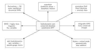
Stochastic currents supplement the ordinary conserved-density theory with fluctuations whose covariance is fixed by dissipative response in equilibrium. An SK formulation supplies normalization, reality, and positivity constraints; dynamical KMS is the extra thermal condition behind fluctuation–dissipation. The other branches require different added variables and must not be generated by reinterpreting this noise sector. The diagram is schematic.
In text: choose a coarse-graining regulator, add conserved noise with covariance , verify the equal-time susceptibility , and distinguish white, colored, and multiplicative noise. This branch extends ordinary hydrodynamics without adding a new conserved density. The other branches require their own additional variables or constitutive structures: for example, a superfluid has a Goldstone phase, while Hydro+ retains extra slow fluctuations that need not be conserved densities.
Exercise
Section titled “Exercise”Verify the equal-time variance above and show what fails if the noise strength is written instead of .
Solution
Using
with gives . Replacing by gives , which has the wrong value and, unless units are hidden in the definition of the noise, the wrong dimensions. The noise pairs with the dissipative mobility ; susceptibility converts that mobility into .
Common pitfalls
Section titled “Common pitfalls”Removing conservation with additive density noise. Conserved noise enters through a divergence unless the source itself represents explicit charge exchange.
Taking the continuum delta function literally. Local variances require a regulator and renormalized parameters.
Attaching Navier–Stokes noise to a causal theory. The response variables and fluctuation kernel must be derived in the same formulation and frame.
Where this leads
Section titled “Where this leads”Schwinger–Keldysh Effective Actions for Fluids generates the diffusion equation and this noise covariance from one action. Long-Time Tails and Fluctuation Renormalization then shows why the nonlinear theory is not exhausted by Gaussian noise.
References
Section titled “References”-
Gavassino, Lorenzo, Nicki Mullins, and Mauricio Hippert. 2024. “Consistent Inclusion of Fluctuations in First-Order Causal and Stable Relativistic Hydrodynamics.” Physical Review D 109: 125002. DOI. Open PDF.
-
Kovtun, Pavel. 2012. “Lectures on Hydrodynamic Fluctuations in Relativistic Theories.” Journal of Physics A: Mathematical and Theoretical 45: 473001. DOI. Open PDF.
-
Landau, L. D., and E. M. Lifshitz. 1987. Fluid Mechanics. 2nd ed. Course of Theoretical Physics, vol. 6. Pergamon Press. DOI.