Initial Correlations and Boundary Terms

Initial correlations are interaction vertices localized on the preparation surface. A Gaussian covariance fixes only one- and two-point data; a correlated interacting state generally has nonzero higher cumulants, which enter the Kadanoff–Baym equations as boundary self-energies and can be required for ultraviolet finiteness and equilibrium stationarity.

Required background. Use the Kadanoff–Baym equations for the bulk evolution and initial density matrices for the contour boundary action.

Helpful background. The numerical validation protocol shows how to separate physical preparation dependence from a discretization transient.

Boundary cumulants in the contour action

In the field basis an initial density matrix can be represented by

$$\langle\varphi_+|\rho_0|\varphi_-\rangle =\mathcal N\exp\!\left\{iS_0[\varphi_+,\varphi_-]\right\},$$

where every field in $S_0$ lies at $t_0$. Expanding with branch indices $a_i\in\{+,-\}$,

$$S_0=\sum_{n\ge1}\frac{1}{n!} \int d^d\mathbf x_1\cdots d^d\mathbf x_n\, \alpha_n^{a_1\cdots a_n}(\mathbf x_1,\ldots,\mathbf x_n) \varphi_{a_1}(\mathbf x_1)\cdots\varphi_{a_n}(\mathbf x_n).$$

$\alpha_1$ fixes the mean, $\alpha_2$ the Gaussian covariance, and $\alpha_{n\ge3}$ encode connected non-Gaussian correlations. Hermiticity, unit trace, and positivity constrain these kernels; arbitrary independent complex coefficients do not define a density operator.

In diagrammatics, an $n$-point boundary kernel is an $n$-leg vertex carrying $\delta(x_1^0-t_0)\cdots\delta(x_n^0-t_0)$. Contracting a boundary four-point vertex with bulk lines contributes an inhomogeneous term to the statistical equation. Schematically,

$$[\partial_t^2+\Omega^2(t)]F(t,t') =I_{\mathrm{bulk}}(t,t')+I_{\mathrm{init}}(t,t'),$$

where $I_{\mathrm{init}}$ contains propagators from $t_0$ to $t$ and $t'$ multiplied by $\alpha_{n\ge3}$. It is not generally representable by changing only $F(t_0,t_0)$.

Equilibrium is the decisive check

Prepare a system in the interacting thermal state and evolve it with the same time-independent Hamiltonian and the same approximation. Every time-translation-invariant correlator should remain stationary. A Gaussian state constructed with a dressed two-point function but no matching higher cumulants can fail this test: the bulk collision term at $t_0$ is not cancelled by its missing boundary partner, producing an “initial slip.”

Garny and Müller derived non-Gaussian initial correlations that restore thermal equilibrium in Kadanoff–Baym evolution and showed how the thermal connected four-point function supplies the leading correction Garny and Müller 2009, §§ 2–4. This is stronger than tuning a Gaussian mass, because it matches the preparation to the same interacting closure.

Ultraviolet structure and double counting

High-momentum correlations must approach a state compatible with the renormalized short-distance theory. A distribution with an arbitrary hard UV tail changes the theory’s energy density and can create divergences unsupported by vacuum counterterms. Conversely, adding a boundary cumulant already generated by an imaginary-time preparation contour double counts the same correlation.

A controlled record therefore specifies:

• whether the state is prepared by a Euclidean leg, an adiabatic source, a quench, or explicit $\alpha_n$ kernels;
• which boundary and bulk counterterms are used;
• how the initial kernels fall at large momentum;
• which correlations are retained at the same order as the bulk self-energy; and
• how observables change when the first omitted cumulant is added.

The relevant acceptance tests appear in the conservation and numerical validation matrix.

The dependency map keeps initial correlations visible all the way to the observable. Its solid arrows carry the boundary density matrix, non-Gaussian cumulants, sources, and memory kernel into the response; the dashed outgoing arrow reserves loss of memory for a separate, observable-specific test.

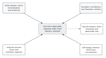
The solid arrows distinguish the inputs to the response calculation from the dashed, separately tested memory-loss conclusion. Non-Gaussian initial cumulants appear as boundary vertices and modify subsequent two-time evolution; they cannot be reproduced merely by choosing a Gaussian propagator. Equilibrium recovery, ultraviolet compatibility, and the absence of double counting must be checked before discarding or absorbing them. The diagram is schematic and not to scale.

The sections Boundary cumulants in the contour action, Equilibrium is the decisive check, and Ultraviolet structure and double counting give the text and equation equivalent of the initial-state dependencies.

Checked weak-correlation example

Let $\rho_0\propto e^{-\beta(H_0+\lambda V)}$. Expanding to first order in $\lambda$ gives

$$\rho_0=\rho_{0,G}\left[1-\lambda\int_0^\beta d\tau\, V_I(-i\tau)+O(\lambda^2)\right]_{\mathrm{connected\ normalization}},$$

where $\rho_{0,G}\propto e^{-\beta H_0}$. For $V=\int\phi^4/4!$, the insertion produces an initial connected four-point cumulant at $O(\lambda)$. Evolving with an $O(\lambda^2)$ scattering self-energy but discarding this $O(\lambda)$ boundary correlation is not a uniform expansion at early times. Including it cancels the corresponding preparation mismatch; it does not alter the canonical $\rho$ sum rule.

Failure tests

Preparation-time test. Move $t_0$ earlier while representing the same physical state. Renormalized later observables should become insensitive once all required boundary data are included.

Stationarity test. Evolve a thermal input with no quench. Drift measures preparation or discretization error, not thermalization.

UV test. Raise the momentum cutoff at fixed renormalized parameters and fixed physical state. A growing early-time spike indicates an incompatible tail or missing boundary counterterm.

Memory-loss test. Vary several admissible preparations with the same conserved densities. Agreement at late times is evidence for loss of selected memory in that model and regime, not a theorem of universal thermalization.

Exercise

Why can an initial three-point cumulant vanish in a $\mathbb Z_2$-symmetric scalar state while an initial four-point cumulant remains necessary?

Solution

The symmetry $\phi\mapsto-\phi$ sets all odd connected correlators, including the three-point cumulant, to zero. It permits even cumulants. Interactions generate a connected four-point function even when the one- and three-point functions vanish, so a Gaussian state can still be inconsistent with the interacting equilibrium closure.

Continue

Track how boundary information propagates through closed-system memory kernels, then verify preparation, cutoff, and timestep stability with numerical Kadanoff–Baym evolution.

References

• Danielewicz, P. (1984). “Quantum Theory of Nonequilibrium Processes, I.” Annals of Physics 152, 239–304. DOI.
• Garny, M., and Müller, M. M. (2009). “Kadanoff–Baym Equations with Non-Gaussian Initial Conditions: The Equilibrium Limit.” Physical Review D 80, 085011. arXiv:0904.3600; DOI.