Memory Kernels in Closed-System Evolution

In a closed interacting system, memory kernels are the time-domain form of nonlocal self-energies: they retain phase coherence and scattering history even though the total evolution is unitary, as emphasized in Berges 2004, §§ 3.4–3.5. Replacing them by a local relaxation time is controlled only when kernel correlations decay on a scale much shorter than every resolved change of the propagators and conserved fields.

Required background. The Kadanoff–Baym equations display the exact causal integration domains.

Helpful background. Open-system memory kernels distinguish bath-induced influence kernels from the collision memory of a closed field theory.

What a closed-system kernel remembers

The statistical equation contains terms of the form

$$I(t,t')=\int_{t_0}^{t}du\,\Sigma_\rho(t,u)F(u,t') -\int_{t_0}^{t'}du\,\Sigma_F(t,u)\rho(u,t').$$

The kernels depend self-consistently on earlier $F$ and $\rho$. They encode off-shell propagation, finite collision duration, coherent oscillations, and initial correlations. Their decay can result from dephasing across a continuum rather than information destruction. In finite volume, recurrences can revive a tail that appeared negligible over a shorter interval.

This is conceptually different from integrating out an environment. A closed-system 2PI kernel transfers information among retained correlation functions within an approximation; an open-system influence kernel results after unobserved degrees of freedom have been traced out. The two may have similar convolution form, but their positivity, noise, and conservation constraints are not interchangeable.

The map identifies memory as a finite-time self-energy convolution attached to the observable, not as an optional narrative term. Its arrows are dependency links rather than a causal-time orientation; the dashed branch is the separate claim that a specified observable has lost sensitivity to earlier times.

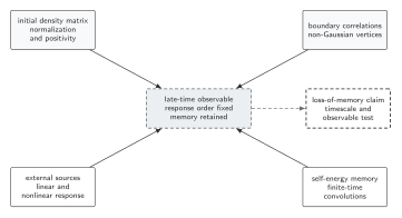
The exact closed two-time evolution retains finite-time memory kernels together with initial and boundary data. Markovianization requires decay and scale separation of the relevant kernel, and a late-time loss-of-memory claim must name both the observable and timescale. It does not follow merely from weak coupling or from replacing a nonlocal kernel by a local rate. The diagram is schematic and not to scale.

The sections What a closed-system kernel remembers, A controlled short-memory expansion, and Conservation-preserving tests provide the text and equation equivalent of the memory dependency and its failure tests.

A controlled short-memory expansion

Consider the exactly localizable convolution

$$M(t)=\int_{0}^{t}du\,\gamma e^{-\gamma(t-u)}x(u).$$

It obeys $\dot M=\gamma(x-M)$ with $M(0)=0$. If $x$ varies on a scale $\tau_x\gg\gamma^{-1}$ and $t\gg\gamma^{-1}$, repeated integration by parts gives

$$M(t)=x(t)-\frac{\dot x(t)}{\gamma} +\frac{\ddot x(t)}{\gamma^2}+O\!\left((\gamma\tau_x)^{-3}\right),$$

apart from the exponentially small initial layer $e^{-\gamma t}x(0)$. The expansion parameter is not “weak coupling” by itself but $\epsilon_{\mathrm{mem}}=(\gamma\tau_x)^{-1}$. For $x=e^{-i\omega t}$, the exact late-time response is $M/x=\gamma/(\gamma-i\omega)$; the local series is the Taylor expansion in $\omega/\gamma$ and fails when $|\omega|\gtrsim\gamma$.

A Kadanoff–Baym kernel need not be positive or monotone. Oscillatory cancellation may make an integral small while its absolute tail remains large, and power-law hydrodynamic tails have no finite correlation time. Therefore a memory window $\tau_{\mathrm{cut}}$ must be validated on observables and conservation residuals, not chosen where the plotted kernel first crosses zero.

From memory to Markovian kinetics

A local collision term additionally requires a Wigner/gradient expansion, loss of sensitivity to the lower boundary, and usually a quasiparticle or controlled finite-width treatment. The logical sequence is

$$\text{two-time kernel} \longrightarrow \text{short relative-time support} \longrightarrow \text{gradient expansion} \longrightarrow \text{on-shell or finite-width closure}.$$

Skipping from the first step to $-\delta f/\tau_R$ introduces an empirical model, not a derivation. A relaxation-time ansatz may be useful, but its conserved zero modes, matching conditions, and range of fitted frequencies must be stated.

Conservation-preserving tests

The conservation and numerical validation matrix applies directly. In particular:

1. compute a reference evolution with the full available history;
2. increase $\tau_{\mathrm{cut}}$ at fixed timestep and total duration;
3. compare unequal-time $F$, $\rho$, conserved energy, and the target observable;
4. repeat after increasing volume, because a finite box changes dephasing and recurrence times; and
5. verify that any local approximation reproduces frequency-dependent response over the claimed band, not merely one fitted decay rate.

Long-time secular error is especially diagnostic. A cutoff may reproduce early damping yet slowly violate energy conservation, shifting the apparent stationary state. Such agreement is transient, not a controlled asymptotic reduction.

Exercise

For the exponential kernel above, find the leading relative error of the Markovian replacement $M(t)\to x(t)$ for $x(t)=e^{-i\omega t}$ after the initial layer.

Solution

The exact ratio is $M/x=\gamma/(\gamma-i\omega)=1+i\omega/\gamma+O((\omega/\gamma)^2)$. The leading complex relative error of replacing $M$ by $x$ is therefore $-i\omega/\gamma$ up to the chosen sign convention for the error. Its magnitude is $|\omega|/\gamma$, confirming that amplitude and phase both require $|\omega|\ll\gamma$.

Continue

The Wigner transformation turns this scale-separation statement into a systematic Moyal expansion. Keep the unreduced two-time result as the benchmark in numerical validation.

References

• Berges, J. (2004). “Introduction to Nonequilibrium Quantum Field Theory.” AIP Conference Proceedings 739, 3–62. arXiv:hep-ph/0409233; DOI.
• Kadanoff, L. P., and Baym, G. (1962). Quantum Statistical Mechanics. New York: W. A. Benjamin. Internet Archive record.