Real-Time Thermal EFT and Dissipative Matching

A real-time thermal EFT must reproduce causal response and fluctuations, not merely a static free energy. Integrating out fast modes on a closed time path produces retarded, noise, and memory kernels whose relations encode unitarity and, in equilibrium, KMS symmetry. A local Langevin or hydrodynamic equation follows only when these kernels admit a controlled low-frequency expansion.

The unitarity, causality, and local-KMS constraints on dissipative Schwinger–Keldysh EFTs are developed by Crossley, Glorioso, and Liu 2017, §§ 2–3.

Required background. Closed-Time-Path Grammar supplies normalized in–in evolution. Thermal Modes, Matching, and EFT Power Counting supplies the hard/slow split. Helpful background. Closed-Time-Path Generating Functionals in Practice develops the $r/a$ basis. System–Environment Splits and Influence Functionals and Schwinger–Keldysh Effective Actions for Fluids develop two important applications.

The quadratic influence action

For a slow bosonic field, define $\phi_r=(\phi_++\phi_-)/2$ and $\phi_a=\phi_+-\phi_-$. After tracing over fast modes, the most general stationary quadratic action can be written schematically as

$$S_{\mathrm{eff}}^{(2)}= \int_{x,y}\phi_a(x)K_R(x-y)\phi_r(y) +\frac{i}{2}\int_{x,y}\phi_a(x)N(x-y)\phi_a(y).$$

Closed-time-path normalization requires $S_{\mathrm{eff}}[\phi_r,\phi_a=0]=0$. Hermiticity relates the action under $\phi_a\to-\phi_a$ and complex conjugation. Causality requires $K_R(x-y)=0$ when $x^0<y^0$. The real symmetric kernel $N$ must define a nonnegative quadratic form so that $e^{iS_{\mathrm{eff}}}$ damps, rather than amplifies, large difference fields.

Matching consists of equating the full and EFT retarded and symmetric two-point functions—or their inverse kernels—in the chosen low-frequency, low-momentum window. Matching only $K_R(0,\mathbf p)$ leaves dissipation and noise undetermined.

Equilibrium ties noise to dissipation

For a time-reversal-compatible equilibrium state, KMS symmetry imposes a fluctuation–dissipation relation. With the displayed inverse-kernel convention,

$$N(\omega,\mathbf p)= -\coth\!\left(\frac{\beta\omega}{2}\right) \operatorname{Im}K_R(\omega,\mathbf p).$$

For $K_R\supset-i\gamma\omega$ with $\gamma>0$, the classical low-frequency limit is $N\simeq2\gamma T$. The corresponding local stochastic equation has damping $\gamma$ and white noise of that strength. This limit requires the bath correlation time to be short compared with the retained evolution time.

Away from equilibrium there is no universal KMS relation. One must match response and fluctuation kernels separately; an “effective temperature” inferred from their ratio can depend on frequency, momentum, and observable.

Memory and the derivative expansion

A local expansion such as

$$K_R(\omega,\mathbf p) =m_{\mathrm{eff}}^2+c_s^2\mathbf p^2 -i\gamma\omega-\tau\omega^2+\cdots$$

is licensed only if the exact kernel is analytic over the frequencies used and no omitted pole or cut approaches the origin. Long-time tails, thresholds, conserved modes, critical slowing down, and pinching singularities generate nonanalytic terms such as $(-i\omega)^{d/2}$ or additional slow poles. Then the correct EFT is nonlocal in time or must retain the newly slow mode explicitly.

A finite Taylor series can also introduce spurious high-frequency poles. These lie outside the EFT only if the claimed frequency range remains well below them and the initial-value problem is treated consistently. Exact causality is a property of the retarded kernel; it cannot be inferred from positivity of a Euclidean quadratic form.

Static and real-time matching answer different questions

The Euclidean zero-frequency action fixes equilibrium weights and static susceptibilities. Under exact analytic assumptions, the full Euclidean correlator at all Matsubara frequencies constrains a unique analytic continuation. A finite set of noisy Euclidean data does not determine the small-frequency spectral shape or a Markovian noise kernel without additional assumptions.

Consequently, a real-time EFT record must state

• the retained slow fields and environmental split;
• the initial state and whether KMS applies;
• the retarded, symmetric, and higher cumulants matched;
• the causal prescription and contour convention;
• the frequency–momentum window;
• memory and derivative-expansion diagnostics; and
• positivity, normalization, and omitted-mode checks.

These entries are summarized in the matching and double-counting table. This page states established quadratic consistency relations; nonlinear and research-specific truncations require model-by-model evidence.

The schematic below organizes the relationships used on this page. Inspect it with this question in mind: How do static and real-time thermal EFTs partition hard, soft, electric, magnetic, and dissipative modes?

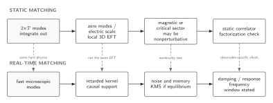
Static reduction integrates frequency-gapped modes into local Euclidean coefficients, while real-time matching fixes retarded, noise, and memory kernels; electric and magnetic sectors can require different retained theories. Solid connections show the primary relation; dashed outlines or arrows mark qualifications and failure boundaries. The diagram is schematic and not to scale.

The surrounding discussion supplies the relevant equations and checks in text form; the figure is a navigational summary.

Exercise

Assume $K_R=-i\gamma\omega$ at low frequency. Use the equilibrium relation to obtain the white-noise limit and explain why it fails when $K_R$ has a branch point at $\omega=0$.

Solution

Since $\coth(\beta\omega/2)\simeq2T/\omega$, the relation gives $N\simeq-(2T/\omega)(-\gamma\omega)=2\gamma T$. A branch point makes the low-frequency kernel nonanalytic, so no finite local derivative expansion captures its memory tail; the noise is generally colored and must retain the same nonlocal structure required by KMS.

References

• Crossley, Michael, Paolo Glorioso, and Hong Liu. “Effective Field Theory of Dissipative Fluids.” Journal of High Energy Physics 2017, no. 9 (2017): 95. doi:10.1007/JHEP09(2017)095.
• Feynman, Richard P., and Frank L. Vernon Jr. “The Theory of a General Quantum System Interacting with a Linear Dissipative System.” Annals of Physics 24 (1963): 118–173. doi:10.1016/0003-4916(63)90068-X.
• Kamenev, Alex. Field Theory of Non-Equilibrium Systems. Cambridge: Cambridge University Press, 2011. doi:10.1017/CBO9781139003667.
• Sieberer, Lukas M., Michael Buchhold, and Sebastian Diehl. “Keldysh Field Theory for Driven Open Quantum Systems.” Reports on Progress in Physics 79, no. 9 (2016): 096001. doi:10.1088/0034-4885/79/9/096001.