Lindblad Field Dynamics and Complete Positivity

A GKSL—or Lindblad—generator is the general generator of a norm-continuous completely positive trace-preserving semigroup in finite dimension. It separates coherent evolution from stochastic jumps and their compensating loss term. For a regulated field theory this form is an invaluable consistency condition, but it does not supply a microscopic bath, prove relativistic causality, or justify removing the regulator.

Required background. Quantum master equations derive the weak-coupling route and distinguish Redfield from secular dynamics. Helpful background. Trace, positivity, and causal consistency gives independent tests beyond recognizing the formal generator.

The GKSL generator

For a density matrix on a finite-dimensional regulated Hilbert space,

$$\dot\rho=\mathcal L\rho =-i[H,\rho] +\sum_{i,j}c_{ij} \left( F_j\rho F_i^\dagger -\frac12\{F_i^\dagger F_j,\rho\} \right),$$

where $H=H^\dagger$ and the Kossakowski matrix $c$ is positive semidefinite. Diagonalizing $c$ produces jump operators $L_\alpha$ and the equivalent form

$$\mathcal L\rho=-i[H,\rho] +\sum_\alpha\mathcal D[L_\alpha]\rho, \qquad \mathcal D[L]\rho=L\rho L^\dagger -\frac12\{L^\dagger L,\rho\}.$$

The anticommutator and recycling terms are not independent choices. Their coefficients are tied so that $\operatorname{Tr}\mathcal L\rho=0$. Positivity of $c$ is what promotes positivity of isolated states to complete positivity under extension by an arbitrary spectator system. The finite-dimensional generator theorem is due independently to Gorini, Kossakowski, and Sudarshan 1976 and Lindblad 1976.

The theorem assumes a time-homogeneous Markov semigroup $e^{t\mathcal L}$. A time-dependent equation in instantaneous GKSL form with nonnegative rates gives a CP-divisible map, but a general CPTP evolution need not be CP-divisible and need not possess such a generator at every time.

Field jumps, regulators, and domains

At a spatial cutoff, one may use local jumps such as

$$L_{\mathbf x}=\sqrt{\gamma}\,\phi_{\mathbf x}, \qquad L_{\mathbf x}=\sqrt{\kappa}\,a_{\mathbf x},$$

or smeared continuum expressions

$$L_f=\int d^dx\,f(\mathbf x)\mathcal O(\mathbf x).$$

Smoothing is not merely numerical convenience. Quantum fields and their composites are operator-valued distributions, so a pointlike $L(x)$, $L^\dagger(x)L(x)$, and its dissipator require a domain, regulator, and usually renormalization. At fixed lattice spacing and finite local occupation cutoff, the finite-dimensional theorem applies directly. With bosonic modes of unbounded occupation or in the continuum, formal GKSL notation is not by itself a proof that a conservative completely positive semigroup exists on the desired state space.

Symmetries constrain the jump set. A conserved charge $Q$ is preserved for all states precisely when the adjoint generator obeys

$$\mathcal L^\dagger Q =i[H,Q] +\sum_\alpha\left( L_\alpha^\dagger QL_\alpha -\frac12\{L_\alpha^\dagger L_\alpha,Q\} \right)=0.$$

It is sufficient, but not necessary, for $H$ and every $L_\alpha$ to commute with $Q$. For gauge theories the generator must preserve the physical constraint algebra; using gauge-variant jumps on an enlarged Hilbert space and projecting afterward need not define the same reduced dynamics.

Spatially local jumps also do not automatically prove relativistic microcausality. The bath correlations, Hamiltonian, regulator, and support of the generator determine propagation. On a lattice, locality can yield a dissipative Lieb–Robinson-type bound; a continuum causal claim requires its own limit and response test.

Why the effective Hamiltonian is conditional

Define

$$H_{\mathrm{eff}}=H-\frac{i}{2}\sum_\alpha L_\alpha^\dagger L_\alpha.$$

Then

$$\dot\rho=-i(H_{\mathrm{eff}}\rho-\rho H_{\mathrm{eff}}^\dagger) +\sum_\alpha L_\alpha\rho L_\alpha^\dagger.$$

For a pure state propagated only by $H_{\mathrm{eff}}$,

$$\frac{d}{dt}\langle\psi\vert\psi\rangle =-\sum_\alpha\langle\psi\vert L_\alpha^\dagger L_\alpha\vert\psi\rangle.$$

The lost norm is the probability density for a detected jump. A quantum-trajectory unraveling alternates nonunitary no-jump propagation with $\lvert\psi\rangle\mapsto L_\alpha\lvert\psi\rangle$, normalized after the jump. Averaging over the records recovers the Lindblad density matrix. Different unravelings can represent the same unconditional generator, so trajectory-dependent entanglement or measurement statements require the monitoring scheme; those information-theoretic questions continue in open and monitored entanglement.

For one decaying field mode, take $L=\sqrt\kappa,a$ and an initial one-particle state. The no-jump branch is

$$\tilde\rho_{\mathrm{nj}}(t)=e^{-\kappa t}\lvert1\rangle\langle1\rvert,$$

whose trace is the probability that no quantum has been emitted. The unconditional solution is

$$\rho(t)=e^{-\kappa t}\lvert1\rangle\langle1\rvert +(1-e^{-\kappa t})\lvert0\rangle\langle0\rvert.$$

Omitting the recycling term therefore does not produce “the same dynamics with loss”; it changes a normalized mixed-state evolution into a postselected, unnormalized branch. Complex optical potentials and quasiparticle widths can remain correct for their declared amplitudes or poles, but they are not unconditional density-matrix generators without the complementary fluctuations or jumps.

Fixed-cutoff guarantee versus microscopic derivation

The GKSL form answers a structural question: given $H$, $L_\alpha$, and a suitable domain, does the time-homogeneous reduced evolution remain CPTP? It does not answer why those operators and rates arise. A microscopic derivation must still specify the bath state and spectral density, the weak-coupling or coarse-graining limit, and the Lamb shift. A phenomenological field generator must instead be matched to observables and supplied with an EFT error estimate.

The chapter’s open-dynamics consistency and evidence matrix distinguishes a fixed-regulator Lindblad model from a microscopic influence trace, a secular weak-coupling limit, and a renormalized open EFT.

Common failure modes

Checking only trace preservation. A trace-preserving Hermiticity-preserving equation can still violate positivity or complete positivity.

Calling every imaginary term a jump. The anti-Hermitian part fixes the total loss operator, but it does not determine a unique recycling channel or measurement record.

Ignoring unbounded domains. Formal cancellation under a trace can fail if $L^\dagger L\rho$ is not trace class or if the chosen state leaves the generator domain.

Assuming the cutoff can be removed. Composite jumps mix with other coherent and dissipative operators. The continuum limit requires counterterms and positivity checks along the flow.

The following reduction map locates a Lindblad field equation within a microscopic open-system argument and separates the full quantum channel from one conditional trajectory.

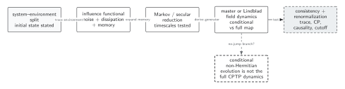
A GKSL-looking expression is the endpoint of controlled approximations, not a guarantee of a continuum quantum field theory. The solid path leads from the system–environment split through the influence functional to the full master equation; the dashed no-jump branch omits recycling terms and is therefore not the complete CPTP evolution. The final checks include operator domains and cutoff dependence in addition to trace preservation and positivity. The diagram is schematic and not to scale.

Equivalently, $H_{\mathrm{eff}}$ governs only the conditioned evolution between jumps, whereas the anticommutator and recycling terms together define the density-matrix map. Composite jump operators must be renormalized, and complete positivity must survive the regulated continuum analysis.

Exercises

For $L=\sqrt\kappa,a$, verify the evolution of the mean occupation.

Solution

Using the adjoint generator, $\mathcal D^\dagger[a](a^\dagger a)=a^\dagger(a^\dagger a)a-\frac12\{a^\dagger a,a^\dagger a\}=-a^\dagger a$. Thus $d\langle n\rangle/dt=-\kappa\langle n\rangle$ and $\langle n(t)\rangle=e^{-\kappa t}\langle n(0)\rangle$.

Let two jumps be collected into a coefficient matrix $c$ with one negative eigenvalue. Can a change of jump basis restore complete positivity?

Solution

No. A basis change transforms $c$ by congruence and cannot change its inertia under an invertible transformation. A negative eigenvalue means the dissipative quadratic form is not positive. One must change the coefficients, the approximation, or the operator set—not relabel the jumps.

Continue to field actions and consistency

Open Schwinger–Keldysh actions translate regulated generators into $r/a$ vertices and response functions. Trace, positivity, and causal consistency tests generators that are not manifestly GKSL, and renormalization of open dynamics asks whether the allowed structure survives changing scale. Condensate, cavity, and circuit realizations continue in driven-dissipative matter.

References

• Breuer, Heinz-Peter, and Francesco Petruccione. The Theory of Open Quantum Systems. Oxford: Oxford University Press, 2002. doi:10.1093/acprof:oso/9780199213900.001.0001.
• Gorini, Vittorio, Andrzej Kossakowski, and E. C. George Sudarshan. “Completely Positive Dynamical Semigroups of N-Level Systems.” Journal of Mathematical Physics 17 (1976): 821–825. doi:10.1063/1.522979.
• Lindblad, Göran. “On the Generators of Quantum Dynamical Semigroups.” Communications in Mathematical Physics 48 (1976): 119–130. doi:10.1007/BF01608499.
• Sieberer, Lukas M., Michael Buchhold, and Sebastian Diehl. “Keldysh Field Theory for Driven Open Quantum Systems.” Reports on Progress in Physics 79 (2016): 096001. doi:10.1088/0034-4885/79/9/096001. Open preprint.